
Think you’re fond of of graphing and computing stuffs? Great! Because you might remember this thing called the Texas Instrument TI-83 from the old days. Sure, while programmable calculators in general are still pretty much popular these days, the graphing calculators from the 21st-century are also coming in waves as we speak — potentially disrupting the market of scientific computing and educational technology.
In particular, there’s a certain education startup out there, relentlessly seeking to hijack our Internet browsers and mobile devices into a — should we say — graphing extravaganza. And it comes with a funky name as well: Desmos.
Yep. You’ve heard it right. As Greek-mythology-inspired as it sounds, Desmos actually has nothing to do with the giant monster responsible for turning Mount Olympus into rubble through the wrath of infernal flames. Instead, it is probably better known as an innocent-looking math tool for the scientifically-minded, making applied math ever more palatable and entertaining!
Oh. Don’t believe in the mighty power of Desmos? Good job! Because it’ll then be our duty to beg to differ, and attempt to convince you otherwise. Indeed, if at the end of the module you still find the scope of Desmos’ functionalities unappealing, then — and only then — shall we concede defeat and return to our ivory tower for more advanced Buddhist meditation training! On the other hand, if you’re just way too lazy to read the 12-page Desmos user manual, and are looking for more concrete examples to kick-start the creative process, then this one is for you too!
Table of Contents
Graphing with Desmos
What is the single word people think of when they hear online graphing calculator? Graphing of course! Indeed, this is something that Desmos does incredibly well — despite having a user interface that appears to be deceptively simple. In what follows, we will see how to we can use Desmos to graph equations, functions and inequalities of different forms, before introducing some bonus features such as graph segmentation, simultaneous graphing and animations!
Equations
When it comes to graphing, equation is one of those first words that comes to mind. On the other hand, it can also be construed as an umbrella term encompassing a plethora of mathematical objects such as explicit functions, implicit functions, parametric equations and polar curves. In what follows, we will illustrate how each of them can be graphed in Desmos — one step at a time.
Preliminaries
Before doing any graphing though, we need to first learn how to type out a few math symbols that are frequently sought for. To that end, we have provided a partial list of common symbols supported in Desmos — along with their associated commands:
- The Multiplication symbol can be obtained by typing
*(Shift+8on US keyboards). - The Division line can be obtained by typing
/(i.e., backslash). - $\pi$ can be obtained by typing
pi, and $\theta$ bytheta. The same goes other Greek Letters such as $\alpha$, $\beta$, $\tau$ and $\phi$. - $\sqrt{}$ by
sqrt, and $\sqrt[n]{}$ bynthroot(after which the value of $n$ can be adjusted manually). - Use the key
^(Shift+6on US keyboards) to create a superscript (e.g., $2$ in $x^2$), and the key_(Shift+Hyphenon US keyboards) for a subscript (e.g., $1$ in $a_1$). - The ceiling function by
ceil(), the floor function byfloor(), and the sign function bysign(). - The absolute value symbol by
|(i.e.,Shift+\on US keyboards).
For some commands (e.g., division, superscript, subscript), typing them out can move the cursor to the upper or lower area. In which case, you can use the arrow keys to help you navigate around the expression and type out what you want. Other times, you might need to use parentheses to group some of your expressions together — before they can be properly interpreted by Desmos.
Defining Functions
Traditionally, the most popular functions are the ones expressed in terms of $x$, which can be typed into a command line as follows:
\begin{align*} y = \text{some algebraic expressions in terms of }x \end{align*}
By reversing the roles of $x$ and $y$, functions in terms of $y$ can also be typed out into a command line as follows:
\begin{align*} x = \text{some algebraic expressions in terms of }y \end{align*}
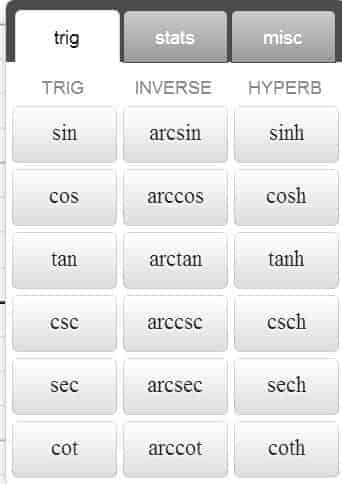
So, what kinds of functions are supported in Desmos? Basically, all of the elementary functions you can think of! These include the 6 basic trigonometric functions, exponential/logarithmic functions (through the commands exp, ln and log), polynomials, and rational functions. In addition, the 6 basic inverse trigonometric functions — along with the 6 basic hyperbolic functions — are readily supported by simply typing out the function’s name as well.
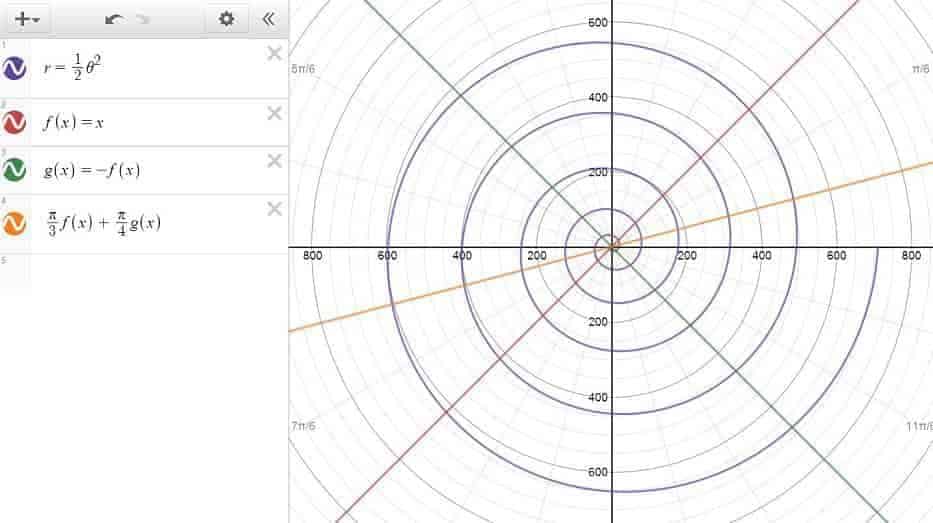
Now, if a function in terms of $x$ is meant to be referred on a repeated basis, then a name can be assigned to it by replacing the $y$ on the left-hand side with, say, $f(x)$. In a similar manner, a function in terms of $y$ can also be assigned a name as well, from which we can define and name a compound function in a command line — without having to resort to rewriting the expressions again and again:
- $y = 2f(3x-3)+e$
- $g(y) = \dfrac{\pi}{f(y)}$
- $f_1(x)= 55f(x)+43g(x) – 100 h(x)$
- $y = g(x)^2 \cdot \left( g(x)^{f(x)} \right)$
- $h(x) = 2 g(f(x)) + 3 g(f(x))$
And in case you’re wondering, the polar functions are equally supported in Desmos as well. However, do note that in this case, the functions will have to be typed out using $r$ and $\theta$ as the designated variables instead (e,g., $r=\frac{1}{2} \theta^2$).
Calculus-Related Functions
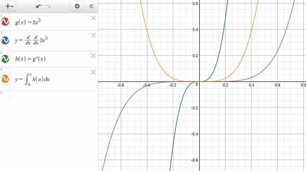
As it turns out, Desmos is remarkably receptive to calculus-based expressions as well. For example, once a function in terms of $x$ is given, by attaching $\dfrac{d}{dx}$ in front of it, the graph of its derivative function can be readily produced — without having to resort to the explicit formula of the derivative. Similarly, the derivative of a function in terms of $y$ can also be graphed by appending $\dfrac{d}{dy}$ in front of it. Pretty neat, right?
Alternatively, if a function has already been assigned a name, we can also use the prime notation to denote its derivative function (as in $f'(x)$). Apart from being easy to implement, the prime notation also has the advantage of being able to refer to higher derivatives by simply adding a few extra $’$ (e.g., $g”$), which — comparing to the repeated use of $\dfrac{d}{dx}$ — is definitely a plus to have.
Of course, if Desmos is good with the derivative functions, then it shouldn’t a surprise that it also supports the integral functions as well. For the record, the integral operator symbol $\int$ can be obtained by typing int into the command line, after which you will have use the arrow keys to navigate around the lower/upper limits and the integrand.
A note of caution though: when setting up an integral function — especially the ones involving multiple integral operators — you want to take that extra care to make sure that the variable of integration is different from the variable(s) in the limits. In doing so, you are in effect removing yourself from the need of punching Desmos for real, in case the expression doesn’t turn out to be exactly Desmos-interpretable. 🙂
Piecewise Functions
To define a piecewise function in Desmos, we can use the following syntax on a command line:
\begin{align*} y \ (\text{or }x) = \{ \text{condition 1}: \text{definition 1}, \text{condition 2}: \text{definition 2}, \ldots \} \end{align*}
As with other functions, a piecewise function can also be given a name by simply replacing the leftmost variable with the name of the function. This way, we can recycle the function repeatedly without having to redefine it ever again.
For example, let’s say that we are interested in defining the function $f$ as the sign function. That is:
\begin{align*} f(x) = \begin{cases} -1 & x<0 \\ 0 & x=0 \\ 1 & x>0 \end{cases} \end{align*}
then this would be the expression we want to type into the command line:
\begin{align*} f(x)=\left\{x<0:-1, x=0:0, x>0:1\right\} \end{align*}
which should produce the following figure:
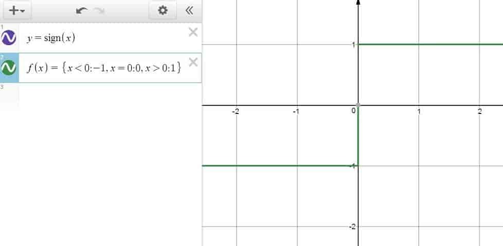
In some occasions, it might be necessary to use the $\le$ and $\ge$ symbols to define a function accurately. In which case, just know that the $\le$ symbol can be obtained by typing out < and = in that order, and the $\ge$ symbol by typing out > and = , again in that order.
Other Equations
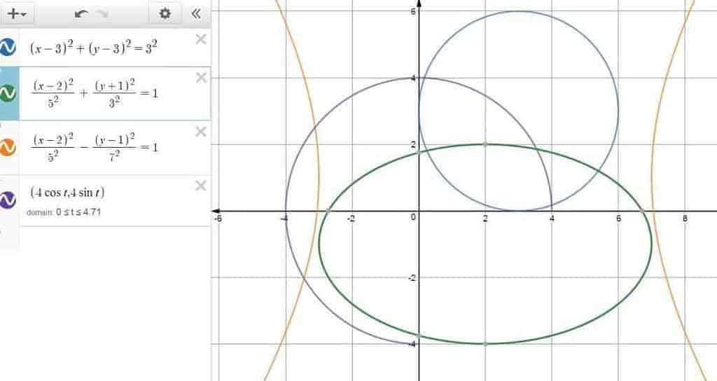
Since Desmos has its interface in Cartesian coordinates by default, it’s only natural that one would use it to plot equations expressed in terms of $x$ and $y$. In fact, implicit functions such as that of a circle, an ellipse or a hyperbola are all very good candidates for this.
However, what is less clear is that Desmos can also interpret parametric equations as well, provided that we type in the equations for $x$ and $y$ as if they were the coordinates of the points instead (as in $(2\cos t, 3 \sin t)$ ), and that the variable $t$ — the designated variable for parametric equations in Desmos — is used throughout the expression. For some reason, Desmos simply won’t take any other variable such as $x$ or $\theta$ for this purpose.
On a more optimistic side, if you manage to type in a parametric equation the right way, then you should be able see an inequality about the domain popping up right underneath the command line. Don’t take this for granted by the way, because this is where you get to configure the range of the variable $t$, which in essence determines the portion of the parametric equations that is actually displayed on the graph.
All right. So far so good? Here’s a figure illustrating how implicit functions and parametric equations work out in Desmos:
Inequalities
Think that was quite a list of equations already? Know this: almost all equations can be turned into inequalities by replacing the $=$ sign with $<$, $>$, $\le$ or $\ge$, thereby easily doubling the amount of graphs one can plot in Desmos. Just a caveat though: don’t do it in a command line where naming the function is precisely the primary goal.
To get it started, here’s a list of inequalities you can try out and get the juice flowing:
- Plane: $y<2x$
- Circle: $x^2+y^2 \le 3^2$
- Inside of a Polar Curve: $r<3\cos ^2\theta$
- Area Between Two Functions (e.g., $f(x) \le y \le g(x)$)
- Space in Between Implicit Functions: $2xy+y^2<4$
And here’s what happened when we throw in these inequalities into Desmos.
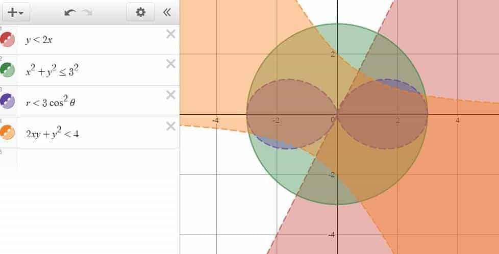
which is pretty cool. And that’s just a start!
Graph Segmentation
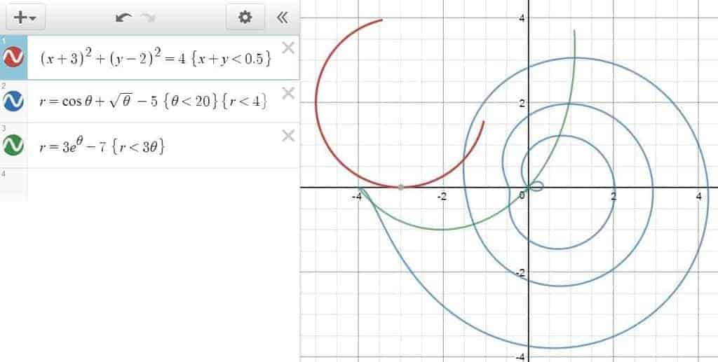
When a valid equation/inequality is entered into a command line, Desmos will — by default — plot its graph by assuming the full domain under which the equation/inequality is satisfied. However, this doesn’t always yield the desired effects, and there are occasions where it’s preferable not to do so. In which case, one can always choose to segment the graph by imposing restrictions on the equation/inequality in question — as long as the following syntax rule is being adhered to:
\begin{align*} \text{equation/inequality} \, \{ \text{condition 1}\}\{ \text{condition 2} \} \ldots \end{align*}
For example, to graph the function $x^2$ with the domain restricted to only the positive numbers, the following line would do:
\begin{align*} y=x^2 \, \{ x>0 \} \end{align*}
Of course, the restriction could have been an inequality on $y$ as well, as in the graph of the function $x^2$ where $y$ is restricted to the interval $[5,15]$:
\begin{align*} y=x^2 \, \{ 5 \le y \le 15 \} \end{align*}
or perhaps an inequality concerning both $x$ and $y$:
\begin{align*} y=x^2 \, \{ x+y<5 \}\{x>0\} \end{align*}
In fact, the restriction(s) could have been any number of equations/inequalities, involving any combination of the designated variables (e.g., $x$, $y$, $r$, $\theta$), with the caveat being that the variables in the restrictions need to be compatible with the equation/inequality they are restricting in the first place (e.g., a polar equation can only be restricted using the polar variables $r$ and $\theta$).
Sounds a bit obscure? Here’s a picture for more info:
Simultaneous Graphing
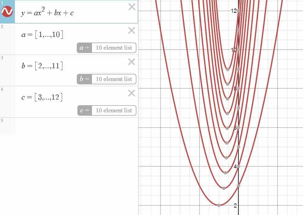
Tired of plotting very similar graphs one by one? Well, despair not, for there is a way out when you’re with Desmos. Indeed, if an equation/inequality is expressed in terms of some parameter(s), which is itself defined as a list of multiple numbers, then multiple graphs can be created simultaneously for each of these numbers once and for all.
Hmm, what are we talking about here? Here’s an accompanying picture to help us out:

As you can see here, by defining a function with the dummy parameter $a$, which is itself defined as a list with the numbers $1$, $2$, $3$ and $4$, we were able to graph a total of four functions simultaneously with a mere two lines. Talk about laziness and efficiency!
And if you’re feeling a bit adventurous, you can certainly try entering an equation/inequality with multiple parameters, each of which is defined as a list on its own with equal sizes. In fact, this “graphing-in-bulk” method has proved to be a formidable technique in drastically slowing down / paralyzing our computers and mobile devices!
On a more serious note though, if you’re looking to exploit the functionalities of Desmos to its fullest, this one is a must. Not only will it automate a graphing process that would otherwise be annoyingly tedious to carry out, but it also prevent us from reinventing the wheel when a template for the graphs is already readily available. Oh, here comes another one!
Animation with Undefined Parameters
When you enter a line of mathematical expression containing an undefined parameter, Desmos will give you to option to include a slider for that parameter, which has the capability of allowing you to adjust of its value manually — or even better yet — create an animation out of it by allowing the value of the parameter to increase/decrease automatically.
In particular, the slider will allow you to control the range and the increment size of the parameter in question, along with the speed and the direction with which the parameter changes. And the reason why it matters, is because by having sliders controlling the behaviors of our parameters of interest, it becomes possible for us to create various animated objects such as movable points, rotating equations and animated regions/boundaries.
For example, to model a particle moving along a sine-wave trajectory, all we need to do is to embed an undefined parameter into the coordinates of the sine wave (as in $(a, \sin 2\pi a)+3$ ), before activating the slider for the parameter using the “play” button. And if the point is meant to be moving along a circular path instead, putting an expression such as $(3\cos a – 5, 3\sin a + 6)$ into the command line would do. Furthermore, if the trajectory of a movable point actually defines a function, then Desmos will automatically make the point draggable across the $x$-axis, making it easier to manipulate than ever!
But then of course, movable points are just one of the many features animation has to offer. For example, if we wish to investigate the contribution of the different parameters of a depressed cubic equation, then we can do so by entering $y=x^3+ax^2+bx+c$ into the command line, before activating the sliders for $a$, $b$ and $c$ in any combination we please. Actually, why not toy around with the sliders a bit first and observe how the shape of the graph changes during this process!
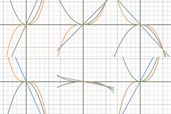
And if instead of having one function change its shape, you are interested in seeing several functions under a common parameter moving all at once, then you can — for example — try typing out $y=ax$, $y=ax^2$, $y=ax^3$ into three command lines, activate the slider, and watch as the polynomials move in tandem with pride!
Computing with Desmos
While the interface of Desmos is primarily composed of a graphing grid than anything else, the fact still remains that it was built fundamentally for computing purpose — and will probably always be. In fact, we will soon see that Desmos — while obviously well-equipped to perform basic computations — can be hijacked into doing a whole bunch of non-graph-related stuffs such as calculating a partial sum, estimating the roots of a function, determining the value of a definite integral, or even finding the greatest common factors from a list of integers!
Elementary Calculations
In Desmos, any mathematical expression involving addition, subtraction, multiplication (*), division (/) and exponentiation (^) can be put into a command line, so that if the expression entered contains no variable whatsoever, then the output can be calculated and returned right back to you — usually in a blink of an eye.
In addition, if some functions such as $f$ and $g$ were already being defined in the command lines and we wish to evaluate an expression involving their function values (e.g., $4f(15)+2g(0)+5$), then we are warranted to type in that same expression into a command line as well, after which Desmos would be more than happy to comply with our request. What’s more, by using the prime notation, we can even get Desmos to evaluate the derivative of a function at a specific point (e.g., $f'(3)$).
By default, when an equation is entered into a command line, Desmos will give us the option to display the key points (e.g., intercepts, local maxima, local minima) on the graph — whenever applicable. Furthermore, if we choose to display these key points, then Desmos will give away the coordinates of these points for free as well — usually up to the first four decimal digits if we just zoom in the graph.
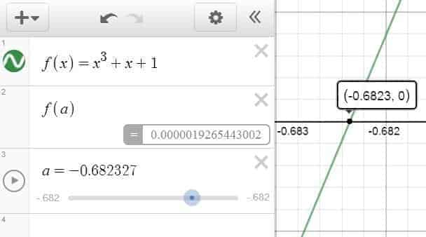
Alternatively, if we are given a function $f$ and we are interested in making a more accurate estimation for the coordinates of a key points (e.g., root finding), we can always try typing in $f(a)$ in a new line and activate the slider for $a$, which in turn allows us to control the value of $a$ manually, and see its effect on $f$ in real-time. In fact, if we just configure the step of the slider to $10^{-6}$ (i.e., the smallest valid increment), then we should be able score a few extra decimals this way.
Furthermore, by naming the mathematical expression we want to compute, we can pass down the output of the computation into a new variable, subsequently using it for other fancier purposes such as building elaborate computations — or graphicalizing the output of the computations into figures and animations.
Lists
When it comes to large-scale computations, it is sometimes more cost-efficient to take the time to construct a list of numbers first, than to manually write down the mathematical expressions one after another. In which case, just know that in Desmos, we can use the square-bracket keys to create a list, whose members could either enumerated explicitly, or implicitly by typing three dots (as in $[7,8, \ldots ,22]$).
In fact, one can also create a list where the members are listed implicitly but with a non-trivial increment (as in $[2,7, \ldots, 42]$), where the increment can be made to be as big as $5635$, or as small as $0.01$ — a flexibility which makes Desmos a powerful tool for defining a large set of numbers.
Note
In Desmos, the square-bracket keys are specifically conceived for the purpose of enumerating the members of a list. For delimiters which serve to group an algebraic expression together, use parentheses instead.
So why exactly do we even bother with creating a list? Because we can use it to run “bulk computations” for each of the members in the list! And if we intend to use a list on a repeated basis, then we can choose to assign a name to the list, and pass the name down into the command lines for even fancier purposes which include, among other:
- Performing a transformation on the list.
- Simultaneously graphing several functions of the same family.
- Plotting a series of points/line/mathematical objects on the graph.
- Calculating the sum of a list — or any other computation which depends on numerically manipulating the members in the list.
All of which are exemplified in the figure below:
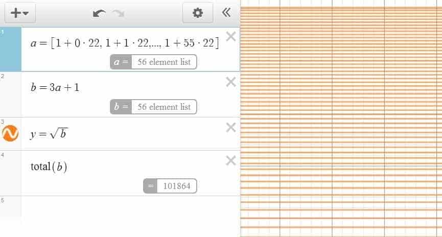
In some occasions, you might it easier to embed the listing and the computations into one single command line, but as the task complexity grows, you might want to consider writing them down in several lines instead to improve legibility and facilitate future references.
Computational Commands
In addition to the standard features offered by a scientific calculator, Desmos has a bit of extra commands available to a typical programmable calculator as well. For example, we can use Desmos to compute the greatest common factor using the gcd command — as long as we adhere to the following syntax:
\begin{align*} \gcd (\text{number 1}, \ldots, \text{number n}) \end{align*}
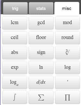
In a similar manner, we can also compute:
- The least common multiple (through the
lcmcommand) - The minimum of multiple numbers (through the
mincommand) - The maximum (through the
maxcommand) - The least positive residue of $a$ under the modulus $b$ (by entering
mod(a,b)) - The number of combinations available when choosing $r$ objects from $n$ objects (by entering
nCr(n,r)) - The number of permutations when choosing $r$ objects from $n$ (by entering
nPr(n,r)) - The factorial of $n$ (by entering
n!)
For example, if your grandpa offers you the chance of choosing 5 giant gummy bears from the 15 that he has to offer, then you can use Desmos to figure out how many ways you can choose the gummies by typing nCr(15,5) into a command line, and be delighted to find out that you actually have $3003$ choices that you can exercise freely. That is, $20+$ times more choices than gummies!
As for the factorial, we’ve got an interesting fact for you: Desmos can calculate the factorial of a number up to $170!$, which is easily more than double of what can be achieved using a TI-83 — or any of its variants for that matter!
Actually, we are not quite done with the computational commands yet. Here’s five more interesting unary operations — for your pleasure:
ceil(): The ceiling function. It allows you to return the ceiling of a number.floor(): The floor function. It returns the floor of a number. Both ceil and floor are relevant in building the staircase functions.round(): The rounding function which rounds a number to an integer.abs(): The absolute value function. Using the vertical bar key|is preferred though.sign(): The sign function discussed a bit earlier, which comes in handy in simplifying some obscure mathematical expressions.
Series
If you look closely at the above figure with the Desmos keypad, you might notice something that looks like a summation sign, along with the Pi product symbol right next to it. Yep. That’s definitely something Desmos can handle for sure!
For example, let’s say that you want to estimate the value of the infinite series $\displaystyle \frac{1}{1^2}+\frac{1}{2^2}+\cdots$, then one of the things you can do is to type something like this into the command line:
\begin{align*} \sum_{i=1}^{1000} \frac{1}{i^2} \end{align*}
For the record, the $\sum$ symbol can be typed out using the sum command, after which you will have to use the arrow keys to navigate around and specify the lower/upper limits. By default, Desmos uses $n$ (instead of $i$, for example) as the main index variable, but you can always change it to another variable at your own discretion — as long as you choose a variable that is not pre-defined for other purposes.
Here, out of curiosity, we decided to toy around with the upper limit a bit, and found that Desmos seems to top out at $9,999,999$ — just one unit short $10$ millions. That’s an astounding improvement from the age of programmable calculators!
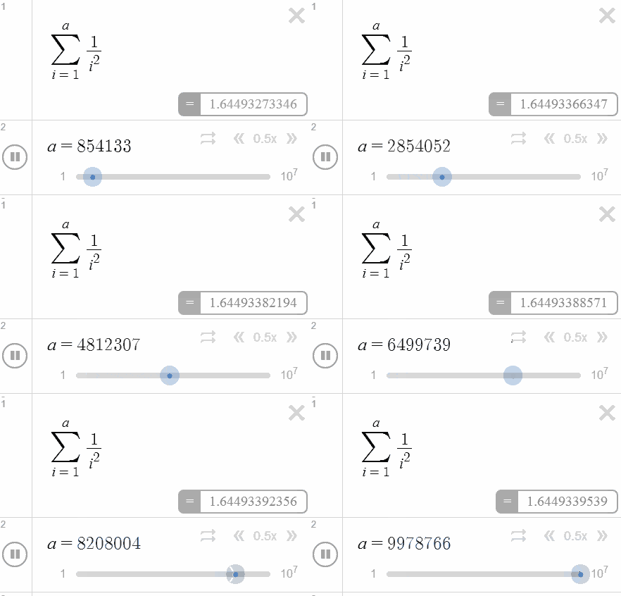
And it gets even better: by using an undefined parameter as the upper limit and configuring the slider accordingly. we get to turn the output of the computations into an animation — as you can see in the figure on the left-hand side. Watch as Desmos showcases its impressive number-crunching power in real-time!
Alternatively, we can also evaluate the product of a sequence using the prod command, and — if needed — stack up as many summations and products as we like. By nesting one operator inside another, we can also evaluate complex mathematical expressions such as those involving double summation or triple product — for instance.
In fact, with just a bit of imagination, we can even turn the result of computations into an animated graph, by converting the numbers into an animated line segment, or — if we so prefer — convert the numbers into a comparative diagram of our liking!
What`s more, the sum and prod commands are not restricted to the computations of numbers either. For instance, we could try plotting out the $n$th-degree Taylor polynomials of $\cos x$ by leaving $n$ as an undefined parameter, so that once we turn on slider with $1$ as the step-size, we should start to see a bunch of functions flashing like crazy!
Definite Integrals
Looking to calculate the area below a strange-looking curve? Struggling to model the total distance traveled by an annoying fly? Or maybe you just want to project your annual revenue for the next year? Either way, the definite integral should have you covered!
In Desmos, the integral symbol $\int$ can be typed out using the int command, after which you can use the arrow keys to navigate around and enter the upper/lower limits. Of course, when defining a definite integral, it’s necessary to include the differential in such a way that the variable of the differential corresponds to the variable in the function you wish to integrate on.
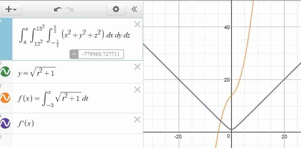
Similar to the cases with the summation and product operators, you are also free to stack up as many integral symbols as you like, and use Desmos to evaluate, say, a double integral (e.g., the volume of a geometrical figure) or even a triple integral (e.g., the total mass of a metal rod). But whichever the case, it’s always a good idea to get into the habit of using parentheses judiciously, so that Desmos understands your expression correctly at each stage of the construction. Otherwise, it’s not our fault if Desmos refuses to parse your expressions like it’s crazy!
So what else can you do with the integral operator? For one, you can try mixing it with summation and product operators, since they are after all the same kind of operator anyway. Alternatively, you can also use integrals to define an equation or an inequality (e.g., integral function), and do all kinds of stuffs with it such as verifying the First Fundamental Theorem of Calculus!
Statistics with Desmos
In addition to the standard graphing/computing features available to most graphing calculators, Desmos also has some neat, native statistical features for the analytically-driven, data-minded individuals. While it’s certainly no replacement for specialized statistical softwares such as R or SPSS, its capabilities in creating/manipulating tables, computing statistical measures and providing regression models should be more than enough to cover the basics for the non-statisticians among us!
Tables
While a list of data forms the basis of univariate statistics, having a table of data with multiple columns opens us to the whole new world of multivariate statistics, a branch of science which is becoming increasingly difficult to ignore in this day and age — where big data and information mining proliferates.
And while you’ll most likely not use Desmos for processing big data involving giant tables and fancy metrics, the fact remains you can still create a table in Desmos through the “add item” menu ($+$ sign in the upper-left corner), and enter the data manually as you see fit. Being primarily a graphing calculator in nature, Desmos seems to prefer presenting a new table with two humble columns by default: the first column $x_1$ presumably for the $x$-values, and the second column $x_2$ for the $y$-values.
Naturally, this setup would lead to the use of table as a way of plotting multiple points of a function, by first filling out a list of input values in the $x_1$ column, followed by redefining the name of the second column as a function of $x_1$ — so that Desmos can learn to automatically fill in the second column all on its own.
Pro-Tip
If you intend to have the values under the first column to be equally spaced, but are too lazy to enter the values yourself manually, then you can auto-fill the first column by pressing Enter repeatedly — after entering the first two values into the column.
In fact, by creating as many columns as we want, we can extend this point-plotting feature a bit to three or four functions simultaneously, All we have to do is to make sure that “function columns” are labeled as a function of $x_1$, and watch as Desmos auto-fills the rest of the table and graph for us. No need to ever redo the $x$-values over and over again!
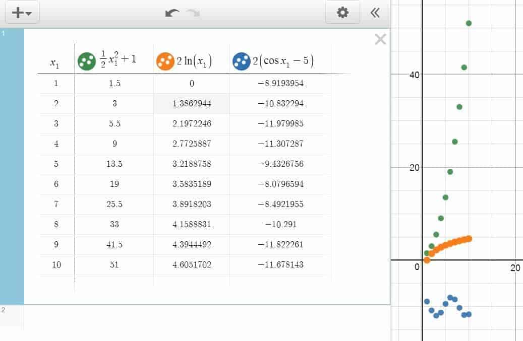
Now, does that mean that you always have to produce a table in Desmos from scratch? Not really. In fact, if you’re familiar any spreadsheet software, you could import the table to Desmos via a simple keyboard copy-and-paste shortcut (Ctrl+C to copy, Ctrl+V to paste). While for a small two-column table, importing data can sometimes be an overkill. For a giant, multi-dimensional table with a dozen of variables, the copy-pasting shortcut can be a true life-saver.
By the way, did you notice the circle icons on the top of most columns? Not only are these icons created every time we create a new column, but they are also our only gateway towards customizing the appearance of the points on the graph as well. By clicking on the gear icon followed by the relevant circle icon, Desmos will give us the option to change the color of the points under the entire column. Alternatively, we can also adjust the graphing style between the points here, by choosing to have either line segments or curves passing through them — a feature which comes in handy for drawing figures or making polygon plots.
To be sure, if you name a column as a function of another pre-existing column, then the values under the new column will be determined by those under the old column. However, if you choose to label the new column as a new variable, then you are in effect making it possible for the entries under the column to assume any numerical value.
(for the record, a new variable doesn’t include any of the pre-defined variables such as $x$ and $y$. However, when you attach a new subscript to a pre-defined variable, it does become a new variable as a result.)
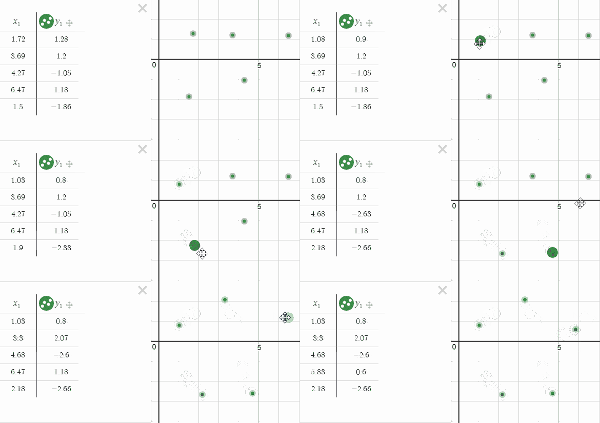
Moreover, for each of the columns that are labeled as a new variable, you can make the points underneath it draggable through the drag setting (accessible again via the gear and circle icons). By configuring the points so that they are either draggable in the horizontal directions, vertical directions, or in every directions, you are essentially giving yourself the choice of manipulating the data visually — which in many cases is more effective than manipulating the data numerically.
Descriptive Statistics
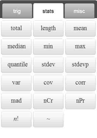
Every time we are given a collection of numbers — either in the form of a list or a column from a table — we can compute some statistical measures based on them. Here’s a list of native, unary statistical commands supported in Desmos:
- Mean: Use the
mean()command to obtain the arithmetic mean of a list of numbers, which can be defined explicitly (e.g., $\mathrm{mean}([2.5,5.7,15,3]) $), or referred to via a variable name (e.g., $\mathrm{mean}(a_1) $). - Median: Use the
median()command to return the middle number (for a set with an odd number of data) or the mean of the two middle numbers (for a set with an even number of data). - Standard Deviation: use the
stdev()command for sample standard deviation, andstdevp()for population standard deviation. - Mean Absolute Deviation: use the
mad()command to find the mean of all absolute deviations of a list. - Variance: use the
var()command to obtain the sample variance. - Total: use the
total()command to find the sum of all numbers in the list. - Length: use the
length()command to find out the number of data in the list. - Extrema: use the
min()command for the minimum, andmax()for the maximum.
Additionally, here’s a list of binary statistical commands supported in Desmos, with slightly more delicate syntax:
- Quantile: To obtain the $p$-quantile of a list $a$, type in
quantile(a,p)into a command line. Note that $p$ must be presented as a decimal between $0$ and $1$. - Covariance: To obtain the sample covariance between the lists $a$ and $b$, type in
cov(a,b)orcov(b.a)into a command line. - Correlation: To obtain the Pearson correlation coefficient between the lists $a$ and $b$, type in
corr(a,b)orcorr(b,a)into a command line.
To be sure, the fact that these are about the only native commands supported in Desmos doesn’t mean that these are the only statistical measures we are restricted to. In fact, we could , for example, evaluate the range of a list $a$ by using the command max(a) - min(a), and calculate the Inter-Quartile Range by using quantile(a,0.75) - quantile(a,0.25).
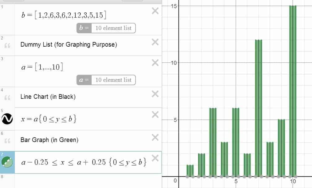
In fact, with just a bit of imagination and ingenuity, it is possible to make out some line charts and bar graphs in Desmos as well. All that is required is some ability in drawing multiple vertical bars and line segments — and perhaps the ability in doing so at the right spots as well. Here’s a figure to keep the idea of data visualization in the loop!
Regression
When looking at a series of points and its associated scatter plot, it’s only natural that we seek to further understand the nature of relationship — if any — between the two variables in question. In which case, it makes sense that we use regression models to explain and predict the behaviors of one variable from another. In fact, if we apply the “right” regression model to the data, we can — more often than not —uncover surprising insights that would have been hard to obtain otherwise.
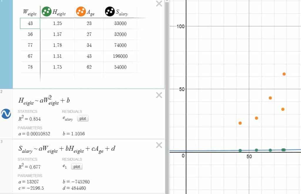
In Desmos, if you have a table with even just two columns — say $x_1$ and $y_1$ — then you can create a regression model for the associated points to your heart’s content. For a linear regression model, just type in $y_1 \sim mx_1 + b$ into a new line, and Desmos will be more than happy to provide a best-fitting line for you. For a quadratic model, you can type in something along the line of $y_1 \sim a{x_1}^2+b x_1 + c$, and a parabola should be ready for you in a blink of an eye. Additionally, if you prefer fitting a higher-degree polynomial instead, or maybe you just find an exponential or a logistic model to be more appropriate, then you are certainly welcome try out those as well — as long as you follow the “regression syntax” outlined a bit above.
What’s more, while the graphing interface of Desmos is built primarily for 2D graphing, that actually doesn’t deter us from doing multivariate regression either. Indeed, if we are given a giant table with 4 columns — says $x_1$, $x_2$, $x_3$ and $y_1$ — then we can fit a linear model for these variables by simply typing something along the line of $y_1 \sim ax_1+bx_2+cx_3 +d$ into the command line, so that even if Desmos is not properly equipped to plot graphs involving multiple independent variables, we can continue to run multivariate regression as if nothing happened in the first place!
Pro-Tip
While a variable name usually takes the form of a single letter in Desmos, we are still free to use as much subscripts as we want to. For example, instead of using P as a variable for population size, we might just as well use Population instead, thereby eliminating the need of guessing what the variable stands for in the near future.
At the end of the day, whichever regression model we choose, Desmos will always be glad to present us with the least-square line for the data, along its parameters (e.g., slope, intercept) and the correlation/$r^2$ of the model. Additionally, we can also use the grey “plot” button (under “residuals” tag) to include the residuals into both the graph and the table — and if we are adventurous enough — pass on the residual variable into the command line again for more detailed analysis!
Miscellaneous
All right. With most of the main features now settled, let’s move on to some other miscellaneous functionalities which you might find useful from time to time. In particular, we’ll see how to use Desmos to tweak around the graph setting, create notes, organizing lines into folders, and make use of the saving and sharing functionalities!
Graph Setting
If you look at the upper-right corner of Desmos’ user interface, you should be able to see an icon with a wrench on it. Why bothers? Because this is the place where you can have access to the Graph Setting menu, which contains a plethora of global setting that one can tweak around for practical and not-so-practical purposes. These include, among others:
- Toggling the grid from rectangular form to circular form — or disabling it entirely.
- Labeling the $x$ and $y$-axes.
- Changing the step size of each axis (e.g., using $\dfrac{\pi}{2}$ as step-size when graphing trigonometric functions).
- Interpreting the angles in either degree or radian.
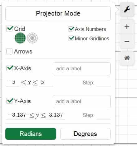
In addition, underneath the wrench icon, you should be able to see a $+$ and a $-$ icon. As one would expect, these icons are used for zooming in and zooming out the graph, respectively, and when either of the features is exercised, you will see beneath the $-$ icon an additional home icon, which allows you to return to the default zoom level. Think of it as some sort of safety net in case you blow up the graph out of proportion (literally)!
Notes
A note is exactly that: a note for yourself and others looking at your graph and command lines. To create a new note, click on the command line where you want the note to appear, then type a " (i.e., the double-quote symbol) to turn the command line into a line for note. While admittedly a non-computational feature, a note can still be used to include any comment, instruction or explanations deemed relevant to the graph and the surrounding computations thereof. In fact, we can even add a few hyperlinks here and there to spice up the discussion a bit. Just remember to start the link with a http or https prefix though.
Collapsible/Expandable Folders
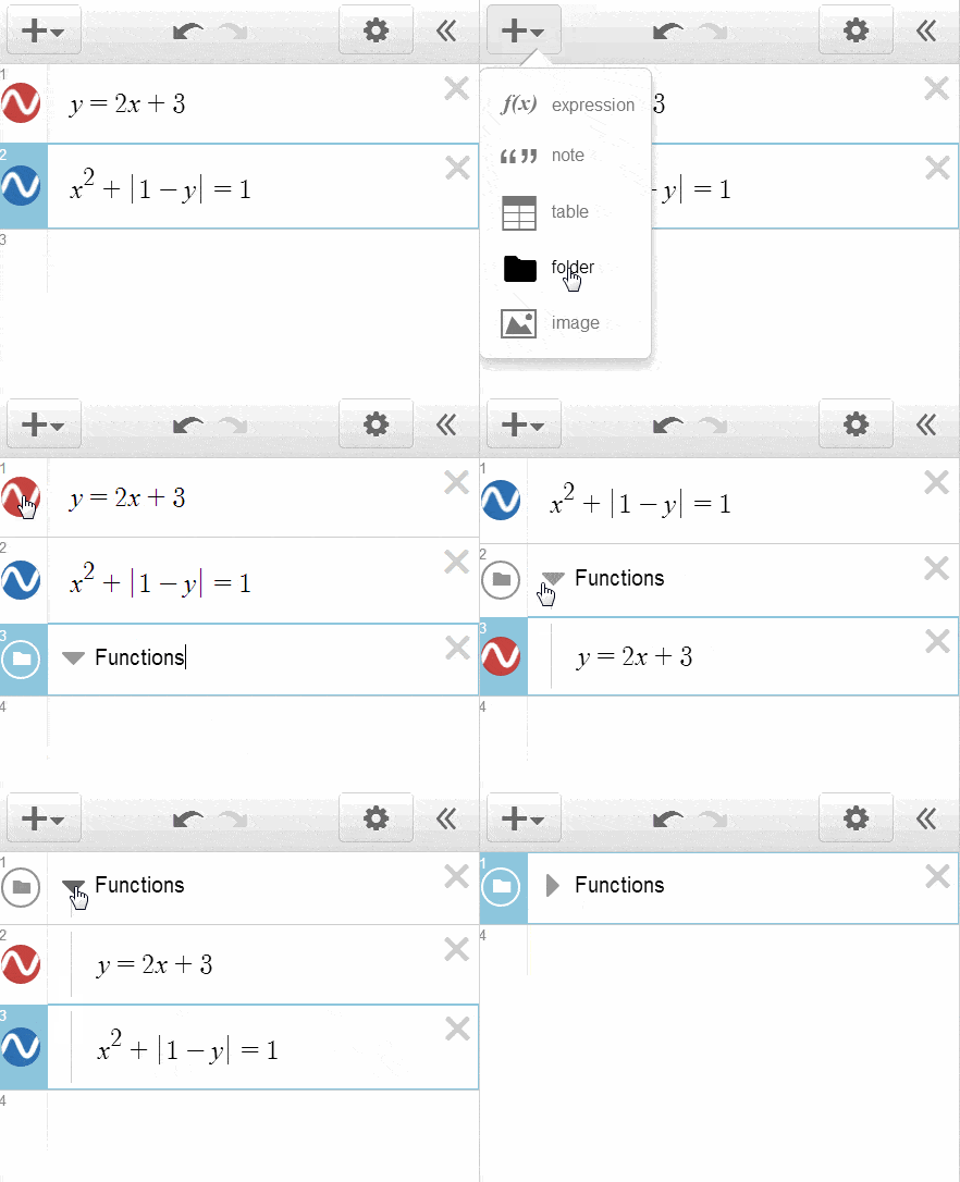
While primarily a cosmetic feature, a folder is integral tool for organizing your command lines into a coherent set of groups — the latter of which can collapsed or expanded upon demand. Similar to the case with a note, a folder can be created by first clicking on the command line where the folder should appear, and then by accessing the Add Item menu via the $+$ icon near the upper-left corner. Once a folder is created, it can be given a label, after which a command line can be dragged in or out of the folder with ease, and the triangular arrow icon next to it can be used to expand/collapse the folder as one wishes.
Images
While graphical calculators are excellent tools for creating geometrical figures, there are certain times where an image goes beyond simple geometry and needs to be imported from somewhere else instead. Fortunately, this is a feature well supported in Desmos, where an image can be added to the graph the same way a folder is added to a command line.
By default, Desmos likes to place an image so that its center is located at the origin, although we can still move/resize the image by dragging along its center or the 8 boundary points surrounding it. In addition, an image’s opacity can be adjusted through the Gear Icon, and its dimensional values / coordinates of the center can also be configured numerically. Heck, we can even sneak in some undefined parameters in them, thereby turning a static image into a flying picture — where the dimension changes from one place to another!
Saving / Sharing Graphs
Find the mighty power of Desmos appealing and intend to use it extensively in the near future? Then it makes sense that you create an account, and work on your graphs while logged into the account. Why? Because then you can actually save these graphs for real, and share them with other like-minded individuals!
In fact, working on a graph while logged in allows you to give a title to the graph, so that if you decide to save it for later, a simple Ctrl + S will do. On the other hand, any saved graph can also be deleted — if needed to — by hitting the $\displaystyle \times$ button next to the name of the graph to be deleted.
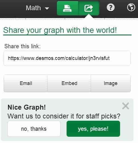
And if you’re feeling generous enough, you can always share your work with others by generating a link for the graph — through the green Share Graph icon near the upper right corner. Remember, Desmos is a cloud-based application after all, which means that every time you save a graph and publish it somewhere online, you are in effect contributing to an ever-growing database of Desmos modules — all in the name of science and technology!
Closing Words
Ouf! That’s quite a bit on an innocent-looking online graphing calculator isn’t it? By the way, if you’ve manage to make it this far, you are already a true hero on your way to becoming a power user of Desmos! At the end of the day, whether you decide to use Desmos for graphing, computing, statistics or other purposes, the hope is that you would find a way to leverage these functionalities and adapt them to your own needs. Who knows, maybe you can even turn some of your inspiration into a fruitful, creative process — with perhaps a bit of technical twist along the way!
All right. Ready for the recap? Here’s a jam-packed interactive table on what we’ve covered thus far:
Preliminaries
| Multiplication |
| Division |
| Greek Letters ($\pi, \theta, \alpha, \beta$) |
| Roots ($\sqrt{}, \sqrt[n]{x}$) |
| Superscript |
| Subscript |
| Ceiling Function |
| Floor Function |
| Sign Function |
| Absolute Value |
| Arrow Keys |
| Parentheses |
Defining Functions
| Functions (in terms of $x$) |
| Functions (in terms of $y$) |
| Trig Functions |
| Exponential Functions |
| Logarithmic Functions |
| Polynomial Functions |
| Rational Functions |
| Inverse Trig Functions |
| Hyperbolic Functions |
| Function Naming |
| Compounding Functions (via $+$, $-$,$\times$, $\div$, $\hat{}$ and $\circ $) |
| Polar Functions |
Calculus-Related Functions
| Derivative Operator |
| Prime Notation |
| Integral Operator |
| Lower/Upper Limits (Integral) |
| Integrand |
Piecewise Functions
| Syntax (Piecewise Functions) |
| Naming a Piecewise Functions |
| Sign Function |
| $\le, \ge$ Symbols |
Other Equations
| Cartesian Coordinates |
| Implicit Equations (e.g., circle, ellipse, hyperbola) |
| Parametric Equations |
| Designated Variable |
| Adjusting the Domain (Parametric Equations) |
| Planes |
| Circles (Inside or Outside) |
| Polar Curves (Inside or Outside) |
| Area (between two functions) |
| Space (in between the implicit functions) |
| Restriction (Syntax) |
| Restriction on $x$ |
| Restriction on $y$ |
| Restriction Involving Both $x$ and $y$ |
| Restriction Involving Other Designated Variables |
| List |
| Dummy Parameter |
| Using Multiple Parameters |
| Undefined Parameter |
| Slider |
| Adjusting Range (Parameter) |
| Increment Size (Parameter) |
| Speed (Parameter) |
| Direction (Parameter) |
| “Play” Button (Slider) |
| Movable Point |
| Multiple Parameters (On a Command Line) |
| Common Parameter (On Multiple Command Lines) |
| Addition |
| Subtraction |
| Multiplication |
| Division |
| Exponentiation |
| Function Values (Evaluation) |
| Derivatives (Evaluation) |
| Key Points (Intercepts, Local Maxima, Local Minima) |
| Displaying Coordinates (Key Points) |
| Root Finding (Using Slider) |
| Naming Expressions |
| Creating a List |
| Explicit Enumeration |
| Implicit Enumeration |
| List Naming |
| List Transformation |
| Simultaneous Graphing (Using List) |
| Plotting Multiple Mathematical Objects (Using List) |
| List-Related Calculations |
| Greatest Common Factor |
| Least Common Multiple |
| Minimum |
| Maximum |
| Least Positive Residue |
| Combination (Counting) |
| Permutation (Counting) |
| Factorial |
| Ceiling Function |
| Floor Function |
| Rounding Function |
| Absolute Value Function |
| Sign Function |
| $\sum$ (Operator) |
| $\prod$ (Operator) |
| Arrow Keys (Navigation) |
| Dummy Variable |
| Upper/Lower Limits (Summation) |
| Animating Series Calculation |
| Nesting Operators |
| Animated Graph (Series) |
| Taylor Polynomial |
| Integral Operator |
| Upper/Lower Limits |
| Differential |
| Double/Triple Integrals |
| Integral Function |
| Table vs. List |
| Creating a Table |
| Plotting Multiple Points on a Function (Table) |
| Creating Multiple Columns (Table) |
| Importing Spreadsheet Data |
| Adjusting Color (for Points in the Table) |
| Graphing Style (Points in the Table) |
| New Variable (as Column Name) |
| Draggable Points |
| Statistical Measures |
| Mean |
| Median |
| Standard Deviations |
| Mean Absolute Deviation |
| Variance |
| Total |
| Length |
| Minimum |
| Maximum |
| Quantile |
| (Sample) Covariance |
| Correlation |
| Range |
| Inter-Quartile Range |
| Line Charts / Bar Graphs |
| Scatter Plot |
| Regression Model |
| Linear Regression |
| Quadratic Regression |
| Higher-Polynomial Model |
| Exponential Model |
| Logistic Model |
| Multivariate Regression |
| Use of Subscripts (Variable Naming) |
| Parameter (Least-Square Line) |
| Correlation / $r^2$ (Least-Square Line) |
| Residual (Least-Square Line) |
| Grid Setting (Rectangular vs. Circular) |
| Labeling Axes |
| Configuring Step Size |
| Angle Setting (Degree vs. Radian) |
| Zoom In / Zoom Out |
| Default Zoom Level |
| Creating a Note (Keyboard Shortcut) |
| Purpose (Note) |
| Adding Hyperlinks |
| Creating a Folder |
| Naming a Folder |
| Adding / Removing Lines from a Folder |
| Expanding / Collapsing a Folder |
| Importing an Image |
| Adjusting Opacity |
| Coordinates of the Center |
| Dimensional Values |
| Moving / Resizing Images (Visually vs. Numerically) |
| Embedding Undefined Parameters |
| Creating an Account |
| Title (Graph) |
| Saving a Graph |
| Deleting a Graph |
| Generate a Link for the Graph |
And with that, this definitive guide on Desmos has now come to an end. Of course, that doesn’t mean that it’s over yet — for there is yet another way to use Desmos which has great aesthetic and pedagogical value, and that is in the creation of computational drawings!


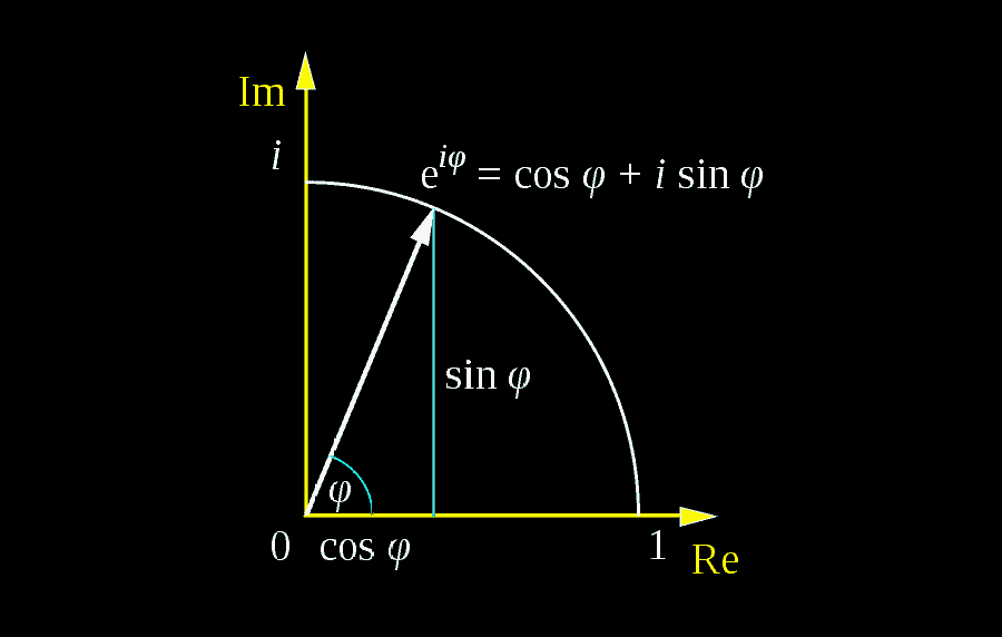
Yeah. It’s pretty cool. Figured out the one with the p-series. 🙂
Yep. You’ve got it. 🙂
As a middle-grade student, my knowledge is basic.
How can I add an x-intercept in Desmos? I need an x-intercept, but I only know how to do a y-intercept and Google is failing me. XD
Hi Rayray. There is no innate function for x-intercept for good reason — because a function or an equation can have 0 or multiple copies of them.
However, all is not lost though, as Desmos will display the coordinates of the x-intercepts if you click on them on the graph. The coordinates are up to a few decimal points of accuracy, and you can type them into the field if you want to.
Impressive way presenting Mathematical Ideas so that more & more of target group can grasp them
easily.
Thank you! Graphing and computing using Desmos is quite a topic all on its own, so we thought that keeping everything under one hood would make people life’s easier!
How can I get more than one decimal place for a slider? I tried to set the step to 0.01, but it does not work.
Hi Yif. It probably depends on how you’re using the parameter. You can adjust the size of step up to 0.000001 by clicking on the cog icon, and you might have to fill in the upper and lower bounds for that to happen.
You can do this by making a slider on the graph.
Define the variable you want to use for the slider, eg "a"
Set lower, upper limit and stepsize eg 0, 10, 0.001
Now define a slideable point: (a,1) and check the label box
The point should now appear in your graph. It might not show all the decimals but if you zoom in on the point to have more accuracy in positioning it, additional decimals will appear. I use this for sliders and switches (0-1). That way I can close the sidepanel and still cotnrol the graph.
Neat idea Frederik. Thanks for sharing!
Great Job!! It's my first time to use it but extremely satisfied with such explanation. This wonderful to us the mathematics teachers/students.
However, what isn't clear enough is how to copy your graph to other areas of work like Microsoft word.
Hi William. Glad that you find the tool useful. If you’re merely looking to copy an unanimated graph to a word processor, you can either use the share icon on the upper right of the Desmos interface to export the graph as an image, or to simply take a screenshot (which can be done natively in both Mac and Windows).