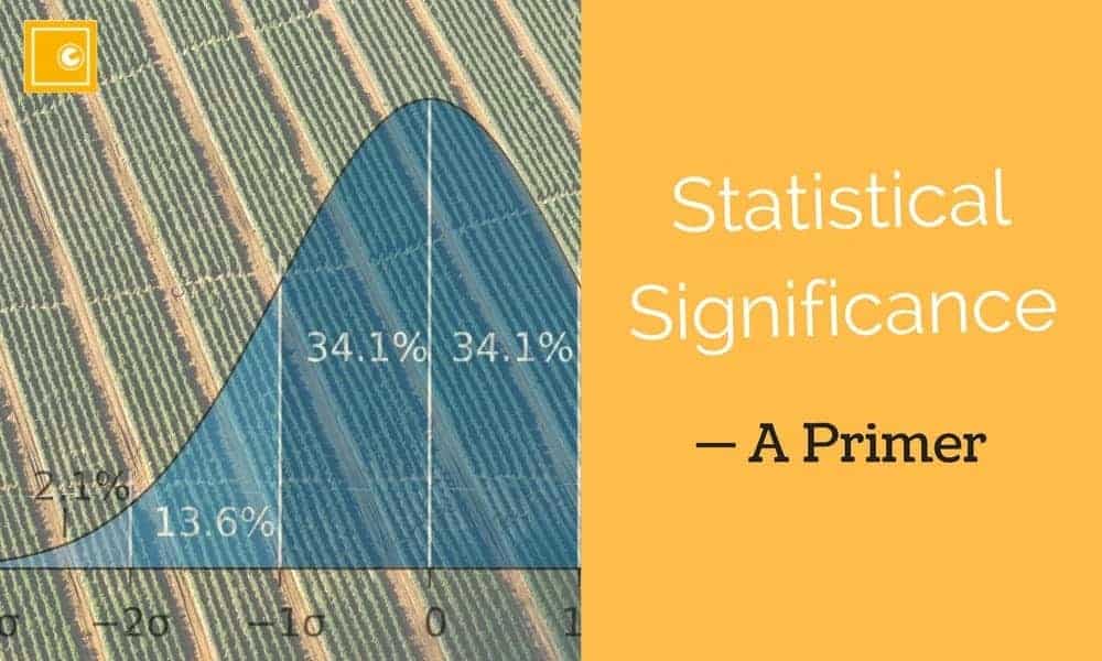
Statistical significance, in a nutshell, is a way of determining the degree of unlikely-ness of an experimental result — when a certain status quo hypothesis is assumed to be true.
For example, let’s say that a school had two teachers, each with approximately $30$ students in their class. Both classes take a standardized test, and it turns out that the average score in class A was $5\%$ better than the average in class B. Statistical significance — in this regard — would be our way of determining whether the better score in class A could be attributed to random chance, for instance:
- It was a lucky day for class A.
- Class A just randomly got assigned better prepared students.
Or whether there is some other factor responsible for the difference in grades between the classes, for instance:
- Teacher A did a better job of teaching than teacher B.
- Teacher A cheated a bit and gave the students some answers ahead of time.
- The classes were purposely split up (e.g., more advanced students or native speakers of a language were put into class A).
Note that in this case, we wouldn’t — using only the information on the scores at least — attempt to decide what the exact reason for the different scores was. Instead, we would just determine if the score difference could be attributed to pure chance, or that it is so unlikely that there might be some other factors involved.
Table of Contents
Getting Started
There are two important things when calculating statistical significance. The first is the magnitude of difference between what you are measuring and what you are comparing against. The second is the amount of natural variation in what you are measuring.
The first concept, magnitude of difference, is easy to understand. Let’s say that you are a farmer growing pumpkins and trying out new fertilizers. You have a baseline average pumpkin weight, which is an average of $10$ lbs. You also have pumpkins from two different fertilizers —A and B — that you are testing out.
If fertilizer A makes pumpkins that weigh $11$ lbs. on average, then it is possible that the $1$ lbs. difference relative to the baseline $10$ lbs. is caused by the fertilizer. However, if fertilizer B produces $25$ lbs. pumpkins on average, then that $15$ lbs. difference ($25-10$) is more likely to be a result of fertilizer B — than the $1$ lbs. difference was to be a result of fertilizer A.
Looking at the Statistical Significance Equation
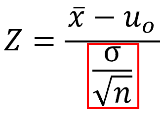
The most commonly used statistical significance test is probably the Z-test. The equation for the Z-test is:
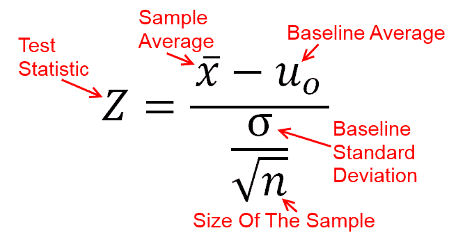
In a nutshell, the Z-Test equation calculates the ratio of two quantities: the numerator on the top, and the denominator at the bottom. Let’s take a look at them individually.
Numerator
The numerator of the equation is where the magnitude of difference is accounted for:

Here, $\bar{x}$ stands for the measured average value for the data set, while $u_0$ stands for the baseline average value. In terms of our example with fertilizer B, the baseline and the measured average would be $10$ lbs and $25$ lbs., respectively, yielding a magnitude of difference of:

In general, the larger in magnitude the final Z-value is, the more significantly the sample deviates from the baseline average value. In particular, having a numerator of $15$ ($25-10$) is more significant than having a numerator of $1$ ($11-10$) — all other variables being equal.
Denominator
So far, we have only been focusing on the top half of the statistical significance equation. Let’s take a look at the denominator of the equation this time:
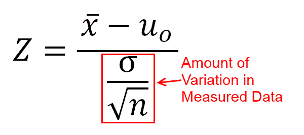
Here, $\dfrac{\sigma}{\sqrt{n}}$ deals with the amount of variation in our measured data. More specifically, the amount of average deviation in the measured averages themselves — if we were to repeat the sampling process indefinitely.
After all, you didn’t think that your pumpkins actually all weighted $25$ lbs. did you? Some probably weighted $22$ lbs., and others $27$ lbs. The $25$ lbs. was just an average, and that measured average could change depending on the pumpkins being sampled.
Normal Curve and Standard Deviation
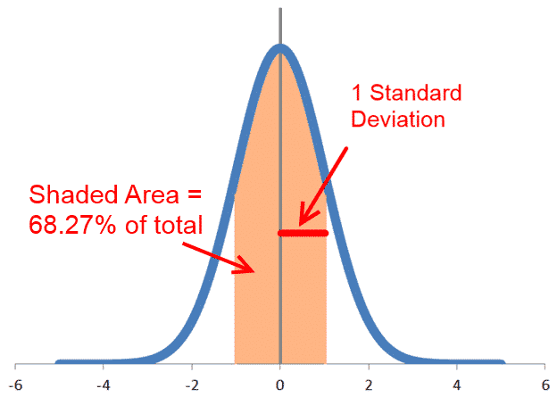
At this point, we need to take a step back and explain what the normal curve and standard deviation are. Loosely speaking, the normal curve is an approximation of how things occur when they are subjected to aggregated, real life random events. The fact that they are random doesn’t mean that they are arbitrary. As a result, they assume the shape of a bell curve as illustrated in the diagram below: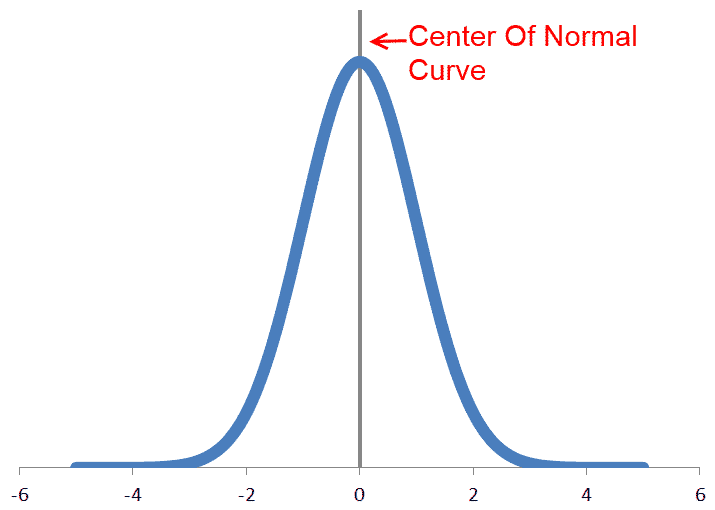 On a related note, the standard deviation is a way of measuring the width of the normal curve, and can be alternately defined as the distance from the center which encloses $68.27\%$ of the area below the normal curve:
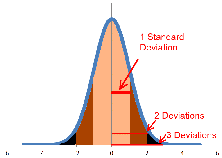
 Similarly, two standard deviations define the distance from the center which encloses $95.45\%$ of the curve, and three standard deviations $99.73\%$ of the curve:
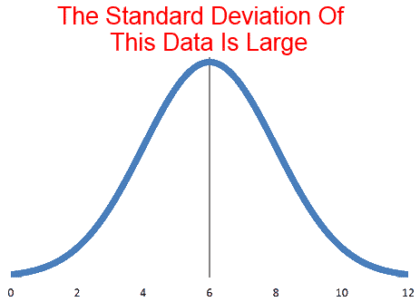
 For a set of data with a lot of variation, the normal curve will be wide, and hence the standard deviation will be large. This would be the case if you take, say, the weight of $100$ rocks you picked up in your backyard.
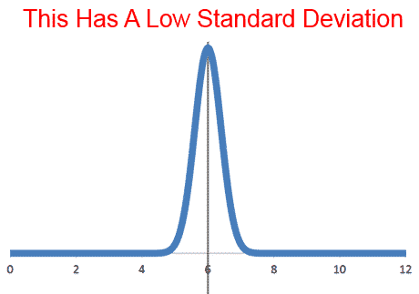
 Or there could also be almost no variation in the data, as in the case where you measured the processing speed for each computer chip in a batch.
 Let’s think about another example — this time involving automobiles. Imagine going to a tire store and being informed that the lifespan of new tires is $50,000$ miles on average, with a standard deviation of $5,000$ miles. Using this information, we can construct the probability distribution of tire lifespan as follows:
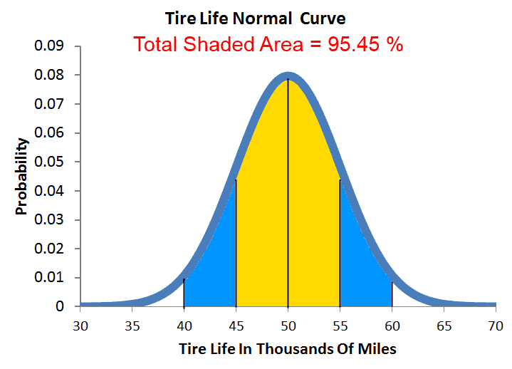
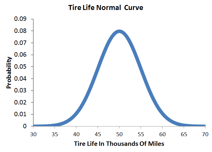 As the graph suggests, we have a $50\%$ chance of being above the average of $50,000$ miles (before needing new tires again), and a $50\%$ chance of being below it. We also know that since two standard deviations correspond to $10,000$ miles (i.e., $5000 \times 2$), we have a $95.45\%$ chance of getting new tires with a mileage between $40,000$ and $60,000$ miles (i.e., two standard deviations within the average):
 Now, let’s say that a couple of years later, you’ve driven $55,000$ miles and your tires are in need of replacement. Would you consider that unusual? No, probably not, since that’s only one standard deviation away from the mean — which is well within the typical tire-to-tire variation often seen in the market.
But now, let’s say that this time you’ve driven $60,000$ miles instead before the tires need replacement. This would be two standard deviations above the average — which is well above the lifespans of most new tires. In addition, since two standard deviations above the average correspond to the top $2.28\%$ of the curve $\left( \frac{100\% – 95.45\%}{2}\right)$, it follows that your tires actually lasted longer than $97.72\%$ of all other tires!
Of course, having a single measurement exceeding $97\%$ of your expected measurements is quite unusual. You have to start thinking, “Maybe there is something different about my situation than the typical installation for the same tires.” For example, it could be that:
- You are just a more cautious driver, and wear down the tires less quickly than the typical person.
- The shop put on better tires than you thought. Maybe you got the next level up by some happy accident.
- The tire company undersells their products a little bit, and it is actually better than they advertised.
Or it could be that it is just a typical variation — and you happen to stumble upon on the right tail of the curve.
Multiple Measurements
So far, we have seen how the normal curve applies to a single measurement. With a single measurement, it is easy to see where it would fall on the normal curve, but how would your opinion change if you had multiple measurements instead?
Maybe you own a fleet of cars, and you got the same type of tires on each of those cars and those tires lasted, say, $46$, $48$, $53$, $54$, $56$, $56$, $57$, $58$, $60$ and $62$ thousand miles. Do these additional measurements make you more or less inclined to believe that the tires last more than the advertised $50,000$ miles?
To be sure, we can, and will, plug those numbers in to the equation to determine the verdict. But there is an interesting reason why the equation works the way it does, and the way to understand it — as luck would have it — is to begin with some dice rolling.
Standard Deviation of Averages
The key to understanding statistical significance is to realize that you actually don’t care much about the standard deviation of the data. What you really care about is the standard deviation of averages — a metric pertaining to samples drawn from the data rather than the data themselves, and which changes as one includes more data into the sample.
Single-Die Rolling
To see how the standard deviation of averages is related to dice rolling, let’s begin our discussion by first throwing a single die. In this case, you have an equal probability of getting a $1$, $2$, $3$, $4$, $5$ or $6$. Here’s the probability distribution of that roll for the record: Here, the average roll you would get is $3.5$, and the standard deviation of the roll — which is the population standard deviation of the set $\{ 1, 2, 3, 4, 5, 6 \}$ — is $1.7078$. Note that the population standard deviation is just a measure of how spread out a data set is, and that the greater a data point deviates from the average in the data set, the more it increases the standard deviation of the data set.
In the case of single die rolling, for example, a roll of a $3$ or a $4$ would contribute the least to the standard deviation. A roll of $2$ or $5$ would contribute a bit more, and a roll of $1$ or a $6$ would be the ones contributing the most.
Two-Dice Rolling
Now, what happens if you roll two dice instead of one, and take the average of those two rolls? For one, you would get $6 \times 6 = 36$ possible outcomes in that case, which correspond to a total of $11$ possible sums — from a sum of $2$ to a sum to $12$.
But here’s the caveat: those $36$ different possible rolls actually don’t map evenly onto the $11$ possible sums! In fact, the most likely sum is a $7$ (which is why casinos win on that roll in craps), while the least likely sum is either a $2$ or a $12$. Here’s the probability distribution for the sum of two dice for the record: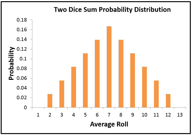 Now, to find the probability distribution for the average of two dice, we just have to take the sums in the above chart, and divide them by $2$. Indeed, if we plot this resulting probability distribution against its single-die counterpart, then we would get a neat graph like the one below:
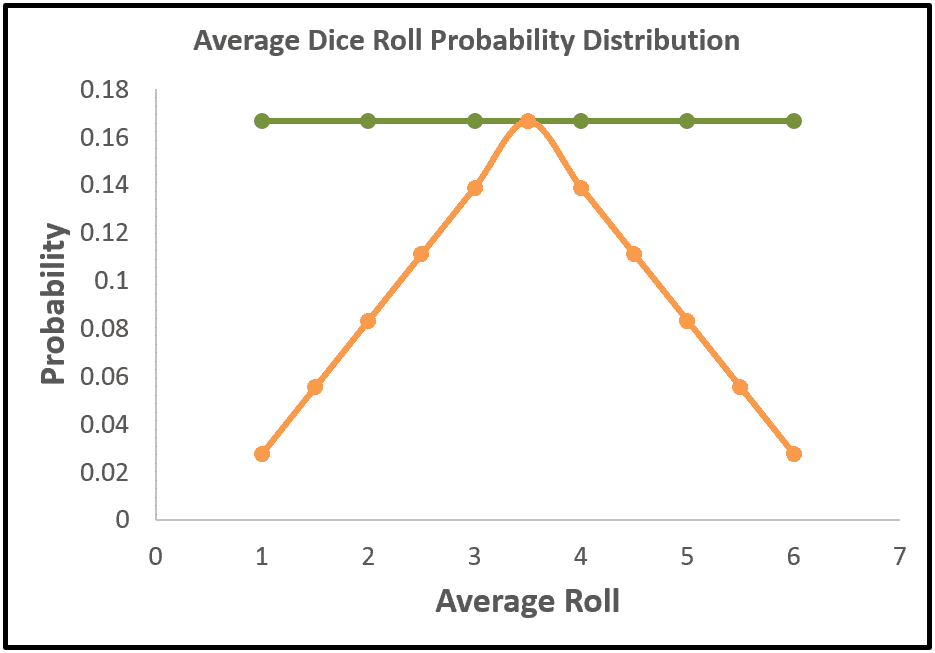 As can be seen from the graph, while the individual probabilities in both distributions sum up to $1$, the shapes of the distributions are actually rather distinct. Granted, both probability distributions do share the same average value of $3.5$, but the two-dice distribution — whose average roll values are spread among twice as many points — generally has lower probability values than its one-die counterpart.
In other words, it’s more likely — with two dice — to get an average closer to the true average of $3.5$, since its probability distribution is generally narrower than the probability distribution with a single die.
Indeed, if we take the standard deviation of the two-dice averages, then we would get $1.2076$, which is smaller than the $1.7078$ we got for the case of one die — again reflecting the fact that the two-dice distribution is less spread out than its single-die counterpart.
Three-Dice Rolling
While we already know that the average-roll distribution of two dice is narrower than its one-die counterpart, what we haven’t seen yet is that this “narrowing” effect is actually more of a general phenomenon. Indeed, if we were to take, say, the average roll of three dice, then we would get an even tighter probability distribution as illustrated in the following graph: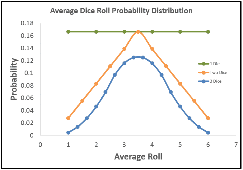 Here, the average of three dice has a standard deviation of $0.986$, which even yet smaller than the one from two dice ($1.2076$), and by extension the one from one die as well ($1.7078$). Alternatively, we can also visualize this decrease from the graph above by observing that the probabilities of getting extreme average rolls (e.g., a $1$ or a $6$) incrementally lessens — as one move from one/two dice to three dice.
(Since the average rolls farthest away from the true average of $3.5$ have an outsized contribution to the standard deviation due to the squaring effect, reducing the probabilities of the extreme average rolls will also reduce the size of the standard deviation itself.)
Multiple-Dice Rolling
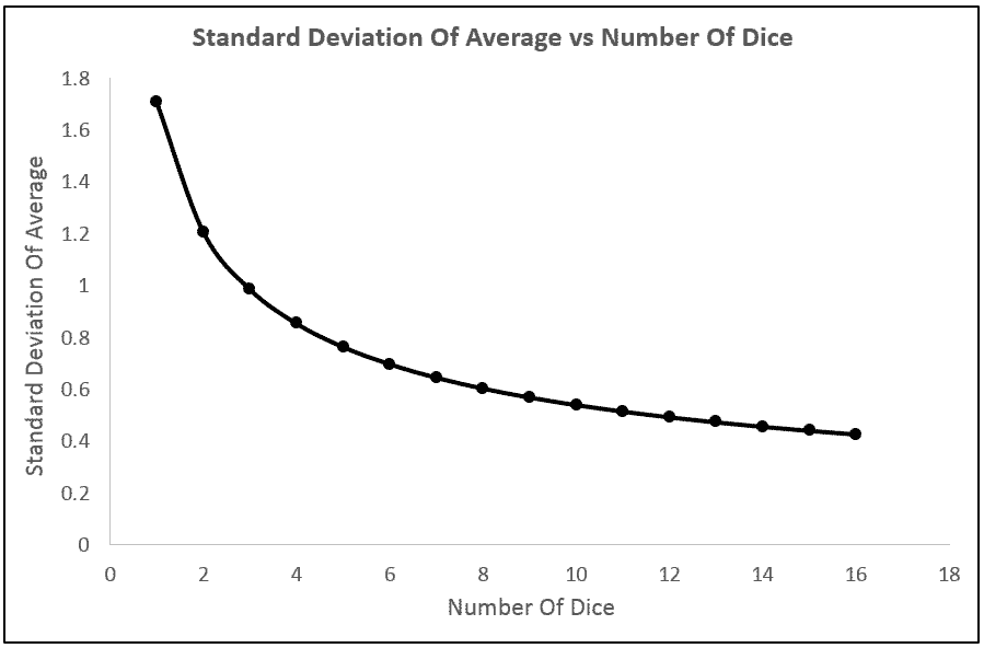
So far, it seems that if we increase the number of dice, the probability of getting an outlying roll decreases as a result. In fact, if we plot the average-roll distributions for $4$, $8$, and $16$ dice against each other, we will see that this “outlier reduction” effect is actually more drastic than the ones we have seen before: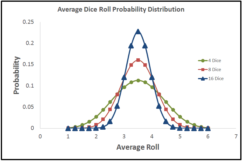 In effect, every time we throw in an additional die into the mix, the standard deviation of average roll would also get reduced by a bit, and if we plot this standard deviation against the number of dice, then we would get a neat graph illustrating this purported inverse relationship:
 And if we put a regression line on this plot, we would get that:
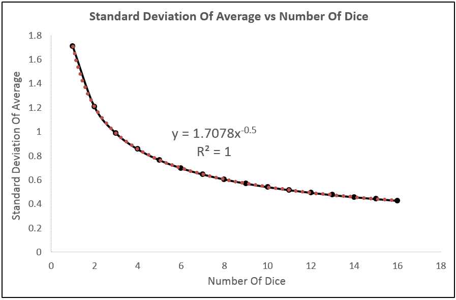 As luck would have it, the regression line is actually an exact fit of all the data! And the regression equation can be rewritten as:
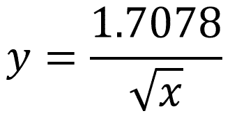 where the numerator is precisely the standard deviation of a single die roll (i.e., population standard deviation).
Now, since $x$ — the number of dice — can be also thought of as the number of data in the sample (i.e., $n$), we see that the above equation is really of the form: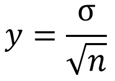 which — if you recall — is precisely the denominator of the Z equation mentioned above!
Relating Dice To Measurements
Although the discussion thus far has been centered around dice rolling, it’s actually not too far-fetch to think of it as drawing samples from a poll of potential values. Indeed, this is exactly what one would do if asked to measure the lifespan of new tires on a car, or the weight of pumpkins from a field.
At the most fundamental level, you have a sample from a pool of possible outcomes, and the more data you include in your sample, the closer the average of the sample will be to the average of the entire pool.
Population-wise, the standard deviation of possible values remains invariant as we increase the data points in our sample. In the case of dice, the population always consists of the values $1$, $2$, $3$, $4$, $5$ and $6$, with its standard deviation remaining at all time invariant at $1.7078$.
Instead, what did change is the standard deviation of averages (of the samples drawn from the population), which incrementally lessens as we increase the size of the sample. And as opposed to the standard deviation of possible values, the standard deviation of averages is really what we are after when it comes to the testing of statistical significance.
What are the Key Points?
- One value that is important to the Z equation is the standard deviation of averages — which is derived from the samples drawn from the population.
- This standard deviation decreases as you draw more data into your sample — since the higher values in the sample are then more prone to being “cancelled out” by the lower values.
- The decrease in this standard deviation is proportional to the square root of the size of the sample.
Back to the Multiple Tire Measurements Problem
In the aforementioned tire example, we originally asked if whether the tires on your car — which lasted for a total of $60,000$ miles — has anything unusual in them. This is under the context where the lifespan of the same tires are assumed to be $50,000$ miles on average, with a standard deviation of $5,000$ miles.
In other words, would the longevity of your tires be the reason to believe that there was something unusual with your car and your tires, or would that be simply the result of a typical random fluctuation which — as it happened — occurred in your favor?
To answer this question, we first determined that at $60,000$ miles, your tires would have lasted two standard deviations above of the baseline average: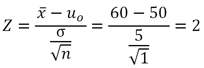 As also established earlier, this would have meant that our tires lasted longer than $97.72\%$ of all other tires, and whether that is unusual enough to suspect another factor at play — other than just random variation — is more of a judgement call than anything.
From there, we continued to ask the same question, but now assuming instead that you actually had $10$ sets of tires on different cars, which lasted $46$, $48$, $53$, $54$, $56$, $56$, $57$, $58$, $60$ and $62$ thousand miles, respectively. Would this additional information increase or decrease your confidence that there was something unusual with the cars or the tires — or that the manufacturer was systematically underrating their product?
Here, the average of our tire lifespans works out to be $55,000$ miles, so it would appear that we would be less confident, since our previous average was $60,000$ miles after all.
However, what we also need to recognize is that we now have $10$ measurements instead of just $1$, so that while the difference in averages went down by a factor of $2$ (i.e., from $60,000 – 50,000 = 10,000$ to $55,000 – 50,000 = 5,000$), the standard deviation of averages also went down by a factor of $\sqrt{10}$ (equiv., $3.162$). Here’s the final Z-statistics for the record: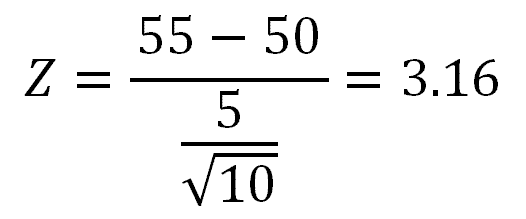 To put it in context, a Z-statistic of $3.16$ means that if the average tire lifespan were actually $50,000$ miles, with a standard deviation of $5,000$ miles, then after taking $10$ measurements, the chance of getting an average value less than the $55,000$ miles we measured, is $99.92\%$.
And since we end up with a higher Z-statistic than before, we are now in an even stronger position to believe that it would be rather unlikely to obtain the unexpectedly high tire lifespan purely as a result of chance.
Closing Remarks
The examples provided here all dealt with the Z-test for statistical significance. The key insight conveyed was that the Z-test equation is designed around the change in the standard deviation of averages (of the samples drawn from a population with a certain possible values), and that this standard deviation of averages decreases as the number of data drawn increases.
Granted, while the Z-test is one of the most commonly used tests for statistical significance, it is certainly not the only one. Also used is the T-test, which is typically applied when less information is known about the baseline population than is required for a Z-test.
Interestingly, despite the fact that some of the T-test equations are more involved, they are all driven by the exact same standard deviation of sample averages. As a result, the same insights provided here also apply to the T-test variations of statistical significance as well.

Thank you for the great article on statistical significance! I appreciate how you used dice rolling and other examples to explain the concepts, and the importance of the standard deviation of averages.
Hi Ana. Glad you find it useful!