Probability and statistics correspond to the mathematical study of chance and data, respectively. The following reference list documents some of the most notable symbols in these two topics, along with each symbol’s usage and meaning.
For readability purpose, these symbols are categorized by function into tables. Other comprehensive lists of math symbols — as categorized by subject and type — can be also found in the relevant pages below (or in the navigational panel).
Table of Contents

Prefer the PDF version instead?
Get the master summary of mathematical symbols in eBook form — along with each symbol’s usage and LaTeX code.
Variables
Probability and statistics both employ a wide range of Greek/Latin-based symbols as placeholders for varying objects and quantities. The following table documents the most common of these — along with each symbol’s usage and meaning.
| Symbol Name | Used For | Example |
|---|---|---|
| $X$, $Y$, $Z$, $T$ | Random variables | $E(X_1 + X_2) =$ $E(X_1) + E(X_2)$ |
| $x$, $y$, $z$, $t$ | Values of random variable | For all $x \in \mathbb{N}_0$, $P(X=x) =$ $(0.25)^x (0.75).$ |
| $n$ | Sample size | $\overline{X}_n = \\ \displaystyle \frac{X_1 + \, \cdots \, + X_n}{n}$ |
| $f$ | Frequency of data | $f_1 + \cdots + f_k = n$ |
| $\mu$ (Mu) | Population mean | $H_0\!: \mu_1 = \mu_2$ |
| $\sigma$ (Sigma) | Population standard deviation | $\sigma_X = \\ \sqrt{\dfrac{\sum (X_i-\mu_x \vphantom{\overline{A}})^2}{n} }$ |
| $s$ | Sample standard deviation | $s = \\ \sqrt{ \dfrac{\sum (X_i-\overline{X})^2}{n-1} }$ |
| $\pi$ (Pi) | Population proportion | $H_a\! : \pi_1 \ne \pi_2$ |
| $\hat{p}$ | Sample proportion | If $\pi_1 = \pi_2$, use $\hat{p} = \dfrac{x_1 + x_2}{n_1+n_2}$ instead of $\hat{p}_1$ or $\hat{p}_2$. |
| $p$ | Probability of success | In a standard die-tossing experiment, $p=\dfrac{1}{6}$. |
| $q$ | Probability of failure | $q = 1-p$ |
| $\rho$ (Rho) | Population correlation | $\rho_{X, X} = 1$ |
| $r$ | Sample correlation | $r_{xy}=r_{yx}$ |
| $z$ | Z-score | $z = \dfrac{x-\mu}{\sigma}$ |
| $\alpha$ (Alpha) | Significance level (probability of type I error) | At $\alpha=0.05$, the null hypothesis is rejected, but not at $\alpha = 0.01$. |
| $\beta$ (Beta) | Probability of type II error | $P(H_0 \,\mathrm{rejected} \mid$ $H_0 \,\mathrm{false}) = 1-\beta$ |
| $b$ | Sample regression coefficient | $y=b_0 + b_1x_1 + \\ b_2x_2$ |
| $\beta$ (Beta) | Population regression coefficient, Standardized regression coefficient | If $\beta_1 = 0.51$ and $\beta_2=0.8$, then $x_2$ has more “influence” on $y$ than $x_1$. |
| $\nu$ (Nu) | Degree of freedom (df) | $\mathrm{Gamma} (\nu / 2, 1 / 2)$ $= \chi^2 (\nu)$ |
| $\Omega$ (Capital omega) | Sample space | For a double-coin-toss experiment, $\Omega = \{\mathrm{HH}, \mathrm{HT}, \mathrm{TH},$ $\mathrm{TT} \}.$ |
| $\omega$ (Omega) | Outcome from sample space | $P(X \in A) =$ $P\big(\{ \omega \in \Omega \mid$ $X(\omega) \in A\} \big)$ |
| $\theta$ (Theta), $\beta$ (Beta) | Population parameters | For normal distributions, $\theta =(\mu, \sigma)$. |
Operators
In probability and statistics, operators denote mathematical operations which are used to better make sense of data and chances. These include key combinatorial operators, probability-related operators/functions, probability distributions and statistical operators.
Combinatorial Operators
| Symbol Name | Explanation | Example |
|---|---|---|
| $n!$ | Factorial | $4! = 4 \cdot 3 \cdot 2 \cdot 1$ |
| $n!!$ | Double factorial | $8!! = 8 \cdot 6 \cdot 4 \cdot 2$ |
| $!n$ | Number of derangements of $n$ objects | Since $\{a, b, c \}$ has $2$ permutations where all letter positions are changed, $!3 = 2$. |
| $nPr$ | Permutation ($n$ permute $r$) | $6P\,3 = 6 \cdot 5 \cdot 4$ |
| $nCr$, $\displaystyle \binom{n}{r}$ | Combination ($n$ choose $r$) | $\displaystyle \binom{n}{k} = \displaystyle \binom{n}{n-k}$ |
| $\displaystyle \binom{n}{r_1, \ldots, r_k}$ | Multinomial coefficient | $\displaystyle \binom{10}{5, 3, 2} = \dfrac{10!}{5! \, 3! \, 2!}$ |
| $\displaystyle \left(\!\!\binom{n}{r}\!\!\right)$ | Multiset coefficient ($n$ multichoose $r$) | From a 5-element-set, $\left(\!\binom{5}{3}\!\right)$ 3-element-multisets can be taken. |
Probability-related Operators
The following are some of the most notable operators related to probability and random variables. For a review on sets, see set operators.
| Symbol Name | Explanation | Example |
|---|---|---|
| $P(A)$, $\mathrm{Pr}(A)$ | Probability of event $A$ | $P(X \ge 5) =$ $1-P(X < 5)$ |
| $P(A’)$, $P(A^c)$ | Complementary probability (Probability of ‘not $A$’) | For all events $E$, $P(E)+P(E’)=1$. |
| $P(A \cup B)$ | Disjunctive probability (Probability of ‘$A$ or $B$’) | $P(A \cup B) \ge$ $\max\left( P(A), P(B) \right)$ |
| $P (A \cap B)$ | Joint probability (Probability of ‘$A$ and $B$’) | Events $A$ and $B$ are mutually exclusive when $P(A \cap B)=0$. |
| $P(A \,|\, B)$ | Conditional probability (Probability of ‘$A$ given $B$’) | $P(A \,|\, B) = \\ \dfrac{P(A \cap B)}{P(B)}$ |
| $E[X]$ | Mean / Expected value of random variable $X$ | $E[2 f(X) + 5] =$ $2 E[f(X)] + 5$ |
| $E[X \, | \, Y]$ | Conditional expectation (Expected value of $X$ given $Y$) | $E[X \,|\, Y =1] \ne$ $E[X \, | \, Y=2]$ |
| $V(X), \mathrm{Var}(X)$ | Variance of random variable $X$ | $V(X) = E[X^2] \, +$ $E[X]^2$ |
| $V(X\, | \, Y), \\ \mathrm{Var}(X \,|\,Y)$ | Conditional variance (Variance of $X$ given $Y$) | $V[X \, | \, Y] =$ $E[\left(X-E[X \, | \, Y] \right)^2 \, | \, Y]$ |
| $\sigma(X)$, $\mathrm{Std}(X)$ | Standard deviation of random variable $X$ | $\sigma(-2X) = \\ |\!-2|\, \sigma(X)$ |
| $\mathrm{Skew}[X]$ | Moment coefficient of skewness of $X$ | $\mathrm{Skew}[X]=$ $\displaystyle E\left[\left(\frac{X-\mu}{\sigma}\right)^3 \right]$ |
| $\mathrm{Kurt}[X]$ | Kurtosis of random variable $X$ | $\mathrm{Kurt}[X]=$ $\displaystyle E\left[\left(\frac{X-\mu}{\sigma}\right)^4 \right]$ |
| $\mu_n(X)$ | nth central moment of random variable $X$ | $\mu_n(X) =$ $E[(X-E[X])^n]$ |
| $\tilde{\mu}_n(X)$ | nth standardized moment of random variable $X$ | $\tilde{\mu}_n(X) =$ $\displaystyle E\left[\left(\frac{X – \mu}{\sigma}\right)^n\right]$ |
| $\sigma(X, Y)$, $\mathrm{Cov}(X, Y)$ | Covariance of random variables $X$ and $Y$ | $\mathrm{Cov}(X, Y) =$ $\mathrm{Cov}(Y, X)$ |
| $\rho (X, Y)$, $\mathrm{Corr}(X, Y)$ | Correlation of random variables $X$ and $Y$ | $\rho (X, Y) = \\ \dfrac{\mathrm{Cov}(X, Y)}{\sigma(X)\,\sigma(Y)}$ |
Probability-related Functions
| Symbol Name | Explanation | Example |
|---|---|---|
| $f_X(x)$ | Probability mass function (pmf) / probability density function (pdf) | $P(Y \le 2) =$ $\displaystyle \int_{-\infty}^2 f_Y(y) \,\mathrm{d}y$ |
| $R_X$ | Support of random variable $X$ | $R_X = \{ x \in \mathbb{R} \mid$ $f_X(x)>0 \}$ |
| $F_X(x)$ | Cumulative distribution function (cdf) of random variable $X$ | $F_X(5)=P(X\le 5)$ |
| $\overline{F}(x), S(x)$ | Survival function of random variable $X$ | $S(t) = 1-F(t)$ |
| $f(x_1, \ldots, x_n)$ | Joint probability function of random variables $X_1, \ldots, X_n$ | $f(1, 2) =$ $P(X = 1, Y = 2)$ |
| $F(x_1, \ldots, x_n)$ | Joint cumulative distribution function of random variables $X_1, \ldots, X_n$ | $F(x, y) =$ $P (X \le x, Y \le y)$ |
| $M_X(t)$ | Moment-generating function of random variable $X$ | $M_X(t)=E[e^{tX}]$ |
| $\varphi_X(t)$ | Characteristic function of random variable $X$ | $\varphi_X(t)=E[e^{itX}]$ |
| $K_X(t)$ | Cumulant-generating function of random variable $X$ | $K_X(t)= \ln \left( E[e^{tX}] \right)$ |
| $\mathcal{L}(\theta \mid x)$ | Likelihood function of random variable $X$ with parameter $\theta$ | If $X \sim \mathrm{Geo}(p)$, then $\mathcal{L}(\theta \mid X = 3) =$ $P(X = 3 \mid p = \theta).$ |
Probability-distribution-related Operators
Discrete Probability Distributions
| Symbol Name | Explanation | Example |
|---|---|---|
| $U \{ a,b \}$ | Discrete uniform distribution from $a$ to $b$ | Let $X$ be the number on a die following its toss, then $X \sim U\{1, 6\}$. |
| $\mathrm{Ber}(p)$ | Bernoulli distribution with $p$ probability of success | If $X \sim \mathrm{Ber}(0.5)$, then $P(X=0) =$ $P(X=1) = 0.5.$ |
| $\mathrm{Geo}(p)$ | Geometric distribution with $p$ probability of success | If $X \sim \mathrm{Geo}(p)$, then $E[X]=\dfrac{1}{p}$. |
| $\mathrm{Bin}(n, p)$ | Binomial distribution with $n$ trials and $p$ probability of success | Let $X$ be the number of heads in a 5-coin toss, then $X \sim \mathrm{Bin}(5, 0.5)$. |
| $\mathrm{NB}(r, p)$ | Negative binomial distribution with $r$ successes and $p$ probability of success | Let $Y$ be the number of die rolls needed to get the third six, then $Y \sim \mathrm{NB}(3, 1/6)$. |
| $\mathrm{Poisson}(\lambda)$ | Poisson distribution with rate $\lambda$ | If $X \sim \mathrm{Poisson}(5)$, then $E[X]=V[X]$ $= 5$. |
| $\mathrm{Hyper}(N, K, n)$ | Hypergeometric distribution with $n$ draws and $K$ favorable items among $N$ | If $X \sim$ $\mathrm{Hyper}(N, K, n)$, then $E[X] = n \dfrac{K}{N}$. |
The following graphs illustrate the probability mass functions of 6 of the key distributions mentioned above.
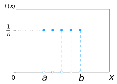
$U\{a, b\}$ 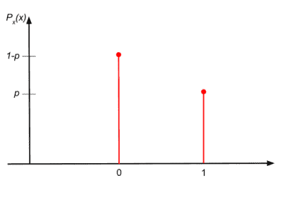
$\mathrm{Ber}(p)$ 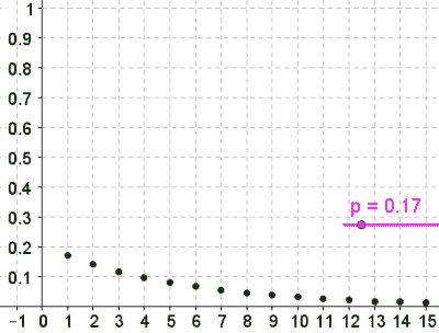
$\mathrm{Geo}(0.17)$ 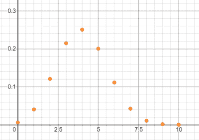
$\mathrm{Bin}(10, 0.4)$ 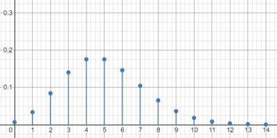
$\mathrm{Poisson}(5)$ 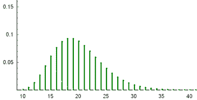
$NB(10, 0.5)$
Continuous Probability Distributions and Associated Functions
| Symbol Name | Explanation | Example |
|---|---|---|
| $U(a, b)$ | Continuous uniform distribution from $a$ to $b$ | If $X \sim U(5,15)$, then $\displaystyle P(X \le 6) = \frac{1}{10}$. |
| $\mathrm{Exp}(\lambda)$ | Exponential distribution with rate $\lambda$ | If $Y \sim \mathrm{Exp}(5)$, then $E[Y] = \sigma[Y] = \dfrac{1}{5}$. |
| $N(\mu, \sigma^2)$ | Normal distribution with mean $\mu$ and standard deviation $\sigma$ | If $X \sim N(1, 5^2)$, then $2X + 3 \sim N(5,10^2)$. |
| $Z$ | Standard normal distribution | $Z \sim N(0, 1)$ |
| $\varphi(x)$ | Pdf of standard normal distribution | $\varphi(x) = \dfrac{1}{\sqrt{2\pi}}e^{-\frac{x^2}{2}}$ |
| $\Phi(x)$ | Cdf of standard normal distribution | $\Phi(z) = P (Z \le z)$ |
| $\mathrm{erf}(x)$ | Error function | $\mathrm{erf}(x) =$ $\displaystyle \dfrac{2}{\sqrt{\pi}} \int_{0}^{x} e^{-t^2} \, dt$ |
| $z_{\alpha}$ | Positive Z-score associated with significance level $\alpha$ | $z_{0.025} \approx 1.96$ |
| $\mathrm{Lognormal}(\mu, \sigma^2)$ | Lognormal distribution with parameters $\mu$ and $\sigma$ | If $Y \sim$ $\mathrm{Lognormal}(\mu, \sigma^2)$, then $\ln Y = N(\mu, \sigma^2).$ |
| $\mathrm{Cauchy}(x_0, \gamma)$ | Cauchy distribution with parameters $x_0$ and $\gamma$ | If $X \sim \mathrm{Cauchy}(0, 1)$, then $f(x)=$ $\dfrac{1}{\pi(x^2+1)}$. |
| $\mathrm{Beta}(\alpha, \beta)$ | Beta distribution with parameters $\alpha$ and $\beta$ | If $X \sim \mathrm{Beta}(\alpha, \beta)$, then $f(x) \propto$ $x^{\alpha-1}(1-x)^{\beta-1}$. |
| $\mathrm{B}(x, y)$ | Beta function | $\mathrm{B}(x, y) =$ $\displaystyle \int_0^1 t^{x-1} (1-t)^{y-1} \mathrm{d}t$ |
| $\mathrm{Gamma}(\alpha, \beta)$ | Gamma distribution with parameters $\alpha$ and $\beta$ | $\mathrm{Gamma}(1, \lambda) =$ $\mathrm{Exp}(\lambda)$ |
| $\Gamma(x)$ | Gamma function | For all $n \in \mathbb{N}_+$, $\Gamma(n)=(n-1)!$. |
| $T (\nu)$ | T-distribution with degree of freedom $\nu$ | $T (n-1)= \dfrac{\overline{X}-\mu}{\dfrac{S}{\sqrt{n}}}$ |
| $t_{\alpha, \nu}$ | Positive t-score with significance level $\alpha$ and degree of freedom $\nu$ | $t_{0.05, 1000} \approx z_{0.05}$ |
| $\chi^2 (\nu)$ | Chi-squared distribution with degree of freedom $\nu$ | $Z_1^2 + \cdots + Z_k^2 = \\ \chi^2 (k)$ |
| $\chi^2_{\alpha, \nu}$ | Chi-squared score with significance level $\alpha$ and degree of freedom $\nu$ | $\chi^2_{0.05, 30} = 43.77$ |
| $F(\nu_1, \nu_2)$ | F-distribution with degrees of freedom $\nu_1$ and $\nu_2$ | If $X \sim T(\nu)$, then $X^2 \sim F(1, \nu)$. |
| $F_{\alpha, \nu_1, \nu_2}$ | F-score with significance level $\alpha$ and degrees of freedom $\nu_1$ and $\nu_2$ | $F_{0.05, 20, 20} \approx 2.1242$ |
Statistical Operators
| Symbol Name | Explanation | Example |
|---|---|---|
| $X_i$, $x_i$ | I-th value of data set $X$ | $x_5 = 9$ |
| $\overline{X}$ | Sample mean of data set $X$ | $\displaystyle \overline{X} = \frac{ \sum X_i}{n}$ |
| $\widetilde{X}$ | Median of data set $X$ | For a negatively-skewed distribution, $\overline{X} \le \widetilde{X}$. |
| $Q_i$ | I-th quartile | $Q_3$ is also the 75th (empirical) percentile. |
| $P_i$ | I-th percentile | $P(X \le P_{95}) = 0.95$ |
| $s_i$ | Sample standard deviation of i-th sample | $s_1 > s_2$ |
| $\sigma_i$ | Population standard deviation of i-th sample | If $\sigma_1 = \sigma_2$, then $\sigma_1^2 = \sigma_2^2$. |
| $s^2$ | Sample variance | $s^2 = \displaystyle \frac{\sum (X_i-\overline{X})^2}{n-1}$ |
| $s_p^2$ | Pooled sample variance | $s_p^2 = \\ \frac{(n_1-1)s_1^2 \, + \, (n_2-1)s_2^2}{n_1 \, + \, n_2-\,2}$ |
| $\sigma^2$ | Population variance | If $\sigma_1^2 = \sigma_2^2$, use pooled variance as a better estimate. |
| $r^2$, $R^2$ | Coefficient of determination | $R^2 = \dfrac{SS_{\mathrm{regression}}}{SS_{\mathrm{total}}}$ |
| $\eta^2$ | Eta-squared (Measure of effect size) | $\eta^2 = \dfrac{SS_{\mathrm{treatment}}}{SS_{\mathrm{total}}}$ |
| $\hat{y}$ | Predicted average value of $y$ in regression | $\hat{y}_0=a + bx_0$ |
| $\hat{\varepsilon}$ | Residual in regression | $\hat{\varepsilon}_i=y_i-\hat{y}_i$ |
| $\hat{\theta}$ | Estimator of parameter $\theta$ | If $E(\hat{\theta})=\theta$, then $\hat{\theta}$ is an unbiased estimator of $\theta$. |
| $\mathrm{Bias}(\hat{\theta}, \theta)$ | Bias of estimator $\hat{\theta}$ with respect to parameter $\theta$ | $\mathrm{Bias}(\hat{\theta}, \theta) = \\ E[\hat{\theta}]-\theta$ |
| $X_{(k)}$ | K-th order statistics | $X_{(n)} =$ $\max \{ X_1, \ldots, X_n \}$ |
Relational Symbols
Relational symbols are symbols used to denote mathematical relations, which express some connection between two or more mathematical objects or entities. The following table documents the most notable of these in the context of probability and statistics — along with each symbol’s usage and meaning.
| Symbol Name | Explanation | Example |
|---|---|---|
| $A \perp B$ | Events $A$ and $B$ are independent | If $A \perp B$ and $P(A) \ne 0$, then $P(B \mid A) = P(B)$. |
| $(A \perp B) \mid C$ | Conditional independence ($A$ and $B$ are independent given $C$) | $(A \perp B) \mid C \iff$ $P(A \cap B \mid C) =$ $P(A \mid C) \, P(B \mid C)$ |
| $A \nearrow B$ | Event $A$ increases the likelihood of event $B$ | If $E_1 \nearrow E_2$, then $P(E_2 \,|\, E_1) \ge P(E_2)$. |
| $A \searrow B$ | Event $A$ decreases the likelihood of event $B$ | If $A \searrow B$, then $A \nearrow B^c$. |
| $X \sim F$ | Random variable $X$ follows probability distribution $F$ | If $X_1, \ldots, X_n \sim$ $\mathrm{Ber}(p)$, then $X_1 + \cdots + X_n \sim$ $\mathrm{Bin}(n, p)$. |
| $X \approx F$ | Random variable $X$ approximately follows probability distribution $F$ | $X_1 + \cdots + X_n \approx$ $N(n\mu, n\sigma^2)$ |
Notational Symbols
Notational symbols are often conventions or acronyms that don’t fall into the categories of constants, variables, operators and relational symbols. The following table documents some of the most common notational symbols in probability and statistics — along with their respective usage and meaning.
| Symbol Name | Explanation | Example |
|---|---|---|
| $IQR$ | Interquartile range | $IQR = Q_3-Q_1$ |
| $SD$ | Standard deviation | $2 \, SD = 2 \cdot 1.5 = 3$ |
| $CV$ | Coefficient of variation | $CV = \dfrac{\sigma}{\mu}$ |
| $SE$ | Standard error | A statistic of $5.66$ corresponds to $10\, SE$ away from the mean. |
| $SS$ | Sum of squares | $SS_{y}= \\ \displaystyle \sum (Y_i-\overline{Y} )^2$ |
| $MSE$ | Mean square error | For linear regression, $\displaystyle MSE = \frac{\sum (Y_i – \hat{Y}_i)^2}{n-2}.$ |
| $OR$ | Odds ratio | Let $p_1$ and $p_2$ be the rates of accidents in two regions, then $OR = \dfrac{p_1 / (1-p_1)}{p_2 / (1-p_2)}$. |
| $H_0$ | Null hypothesis | $H_0\!: \sigma^2_1 = \sigma^2_2$ |
| $H_a$ | Alternative hypothesis | $H_a\!: \rho > 0$ |
| $\mathrm{CI}$ | Confidence interval | $95\% \, \mathrm{CI} = \\ (0.85, 0.97)$ |
| $\mathrm{PI}$ | Prediction interval | $90\%\, \mathrm{PI}$ is wider than $90\% \, \mathrm{CI}$, as it predicts an instance of $y$ rather than its average. |
| $\mathrm{r.v.}$ | Random variable | A r. v. is continuous if its support consists of a union of disjoint intervals. |
| $\mathrm{i. i. d.}$ | Independent and identically distributed random variables | If $X_1, \ldots, X_n$ are i.i.d. with $V[X_i]=\sigma^2$, then $V[\overline{X}] = \dfrac{\sigma^2}{n}$. |
| $\mathrm{LLN}$ | Law of large numbers | LLN shows that for all $\varepsilon >0$, as $n \to \infty$, $P\left(|\overline{X}_n-\mu|>\varepsilon\right) \to 0.$ |
| $\mathrm{CLT}$ | Central limit theorem | By CLT, as $n \to \infty$, $\dfrac{\overline{X}_n-\mu}{\sigma / \sqrt{n}} \to Z$. |
For the master list of symbols, see mathematical symbols. For lists of symbols categorized by subject and type, refer to the relevant pages below for more.
- Arithmetic and Common Math Symbols
- Geometry and Trigonometry Symbols
- Logic Symbols
- Set Theory Symbols
- Greek, Hebrew, Latin-based Symbols
- Algebra Symbols
- Probability and Statistics Symbols
- Calculus and Analysis Symbols

Prefer the PDF version instead?
Get the master summary of mathematical symbols in eBook form — along with each symbol’s usage and LaTeX code.
Additional Resources
- Definitive Guide to Learning Higher Mathematics: A standalone, 10-principle framework for tackling higher mathematical learning, thinking and problem solving efficiently
- Ultimate LaTeX Reference Guide: Definitive reference guide to make the LaTeXing process more efficient and less painful
- Biostatistics for Health Science — Review Sheet: A summary of an entire semester of introductory biostatistics in 5 pages
- Definitive Glossary of Higher Math Jargon: A tour around higher mathematics in 106 terms

This is a heck of a guide!
Thank you Kubet. Glad you like it!